1990issue C121-7
Constructing least-squares polynomial smoothers
A least-squares polynomial smoother is a local linear-regression fit. Place it beside a moving-average baseline and an exponential-smoothing baseline, then size the window by reading leftover structure in the residual series.
- A least-squares smoother is a linear-regression fit that minimizes squared vertical gaps between observed prices and the fitted curve, assigning all error to the price axis and none to the time axis.
- A long moving average reduces extreme peaks and troughs, while exponential smoothing and other asymmetric weighting schemes introduce some shape distortion relative to a symmetric least-squares fit.
- The fitted midpoint can be obtained from an integer-weight window; tabulated sets cover second- through fifth-order polynomials and windows from 5 to 25 observations.
- Window length is a construction choice that should follow inspection of leftover structure in the residual series, because a longer window can add phase delay and change what variation remains.
A linear-regression construction
A least-squares smoother is built as a linear-regression fit. The fit chooses coefficients so the squared vertical gaps between observed prices and the fitted values are minimized. All error is assigned to the price axis and none to the time axis.
Polynomial order is the degree of that local fitted curve. The construction requires evenly spaced sampling and a series that is continuous enough to treat as a smooth curve.
Moving-average and exponential-smoothing baselines
Place this construction beside two baselines that use the same ordered observations. A moving average averages a block of those observations. When that block is long, it tends to flatten sharp peaks and troughs and, relative to the least-squares construction, a long moving average reduces extreme peaks and troughs.
Exponential smoothing applies decaying, asymmetric weights. Relative to a symmetric least-squares fit, exponential smoothing and other asymmetric weighting schemes introduce some shape distortion and shift the shape of turning points.
An integer-weight window
The fitted midpoint can be obtained by multiplying a window of observations by a fixed integer weight set and dividing by a published normalizing factor. That integer-weight window is a compact implementation of the polynomial fit.
Tabulated sets cover second- through fifth-order polynomials and windows from 5 to 25 observations. Second- and third-order sets form one tabulated family, and fourth- and fifth-order sets form another.
The five-point second- and third-order weight set is symmetric about its midpoint and expands from the folded table as -3, 12, 17, 12, and -3.
Sample series versus five-point centered least-squares fit
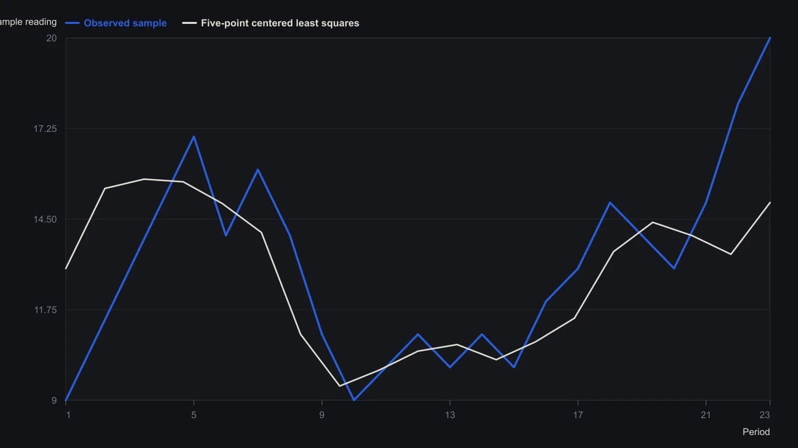
Centered values use the five-point quadratic/cubic integers −3, 12, 17, 12, −3 divided by 35. Periods 1–2 and 22–23 have no centered fit because the window needs two observations on each side.
Five-point and 25-point windows on weekly yields
On weekly intermediate-term bond yields from 6 March 1987 through 12 January 1990, a five-point second- and third-order smoother kept the main highs and lows nearly in phase with the raw series, including the week-34 peak tied to the 19 October 1987 market reaction.
The matching 25-point second- and third-order smoother delayed tall, sharp peaks and troughs by about two to three weeks. That later appearance of the same turns is phase delay. The longer window also spread the week-34 peak toward later observations and left shallow turns near weeks 66 and 110 without that delay.
What the residual series removed
The residual series is the pointwise difference between the raw observations and the smoothed series. It shows how much variation was removed and whether leftover structure remains.
The five-point residual removed about plus or minus 0.1 percent yield at the week-34 spike, confined that burst to about four weeks, and otherwise left background fluctuations near plus or minus 0.03 percent yield plus a roughly regular plus or minus 0.05 percent jump every 17 to 25 weeks.
The 25-point residual removed about plus or minus 0.3 percent yield at the same spike, raised background residual amplitude to about plus or minus 0.1 percent yield, stretched that peak residual toward week 50, and showed a larger leftover oscillation near 30-week spacing.
Sizing the window from leftover structure
Window length is a construction choice that should follow inspection of leftover structure in the residual. After that inspection, the smoother can sit in front of later analysis as a way to decide how much variation, and of what kind, to remove.
All readings on this track · 43 readings
- 1990Constructing dollar baselines from rates, inflation, and residuals
- 1990Constructing a nominal index value from forward earnings and fitted yield
- 1990Constructing a nominal index price from earnings and a fitted yield
- 1990Endpoint-pinned price paths are not forecasts
- 1990Constructing least-squares polynomial smoothers
- 1991Endpoint growth rates versus linear-regression consistency
- 1991Out-of-sample checks for linear growth fits
- 1991Trend as persistence, not a straight line
- 1991Quadratic trend, residual oscillator, and a secondary cycle calendar
- 1991Time-origin offset and residual-price divergence on a quadratic least-squares fit
- 1991A least-squares trendline from ordered prices
- 1992Constructing log-linear growth and reliability screens
- 1992Constructing log-linear growth-rate baselines
- 1992Next-session high, low, and close from rolling linear regression
- 1993Auditing an index price-earnings multiple with short-rate regression
- 1994Regression-seeded nested exponential price filter
- 1994Constructing the double exponential average from lag cancellation
- 1994Evaluating money supply as a linear leading-index baseline
- 1995Constructing least-squares trend channels
- 1995Linear baseline holdout checks for annual bill-rate forecasts
- 1995Projection bands from high and low regression slopes
- 1995Evaluating a least-squares end-point moving average on a known test series
- 1996Constructing an endpoint moving average from a least-squares line
- 1996Scoring equity path consistency with a k-ratio overlay
- 1996Evaluating month-end yield gaps for equity regimes
- 1996Constructing session-indexed standard error bands
- 1998Evaluating linear regression baselines for index valuation
- 1998R-squared as a two-state trend filter from a price-time fit
- 2000Second-order moving-average lag correction
- 2002Price regression line versus beta for index tracking
- 2003Regression slope with an r-squared trend confidence gate
- 2003Constructing finite-volume-element divergence with slope comparison
- 2004Building a daily score from regression, retracement, and volume
- 2004Constructing least-squares trendlines from ordered prices
- 2007Rectangle breakout targets beyond height
- 2007Confirming a price trend with regression slope and r-squared
- 2008A linear-regression angle assembled as one trend filter
- 2010A two-state swing machine from four running extremes
- 2016Score oil-complex tightness before divergence or regression
- 2017Nikkei-yen intermarket divergence as a regime case study
- 2017Constructing Calmar ratio and linear regression baselines
- 2019Pair-trade layer construction versus average-spread management
- 2020A convolution slope built from nested linear regression