1996issue C081-12
Evaluating month-end yield gaps for equity regimes
A historical intermarket-regime-filter classified S&P 500 months from a month-end Treasury yield-gap. The evaluation locked that signed gap, reran the same cash switch with lagged closes, and then converted the gap into a split-sample-linear-fit instead of treating a binary equity-or-cash switch as proof.
- Lock the yield-gap at month-end closes against a six-month-arithmetic-average so the intermarket-regime-filter uses one signed difference for both direction and strength.
- Rerun the rising-yield-state cash switch as a lagged-yield-implementation, because a same-month yield close is not known until month-end.
- Keep the yield-gap continuous in a split-sample-linear-fit and judge the predicted-monthly-change on unseen months rather than collapsing the gap into a binary switch.
- Editorial view: averages by yield state describe association in the archive sample. They do not replace an out-of-sample linear forecast.
Editorial frame: treat this archive note as an evaluation drill for an intermarket-regime-filter. Lock an objective month-end yield-gap, rerun the same cash-switch rule with lagged closes, and then convert that gap into a split-sample linear forecast instead of treating a binary cash switch as proof.
A locked month-end yield-gap
The evaluation used month-end S&P 500 closes from 1950 through 1995 and recorded only close-to-close monthly percentage change, omitting highs, lows, and dividends.
Yield trend was defined by comparing the month-end 30-year Treasury yield with a six-month-arithmetic-average of month-end yields rather than a 120-day daily average. The yield-gap is that signed difference, and it was used both as the direction of the yield trend and as a gauge of its strength.
How months differed by yield state
Across the sample, an average S&P 500 month rose 0.74% and finished higher 57% of the time. Months with the yield below its six-month-arithmetic-average averaged 1.56%, near-average months 1.43%, and months with the yield above the average lost 0.70%.
Those splits describe how equity months lined up with the sign of the yield-gap. They do not, by themselves, test a trading rule or a forecast.
The binary cash switch and look-ahead
A binary intermarket-regime-filter treated a rising-yield-state as a month in which the 30-year yield stood more than 0.1 percentage points above the six-month-arithmetic-average. In that state the hypothetical book moved from equities into cash represented by the 90-day Treasury yield.
Because a same-month yield close is not known until month-end, the same cash-switch rule was also run as a lagged-yield-implementation on last month's close and on the average of this month's and last month's closes. That second pass is the look-ahead check: the filter cannot be allowed to use a close that arrives only when the month is already over.
Cash switch when the 30-year yield gap exceeds 0.1%
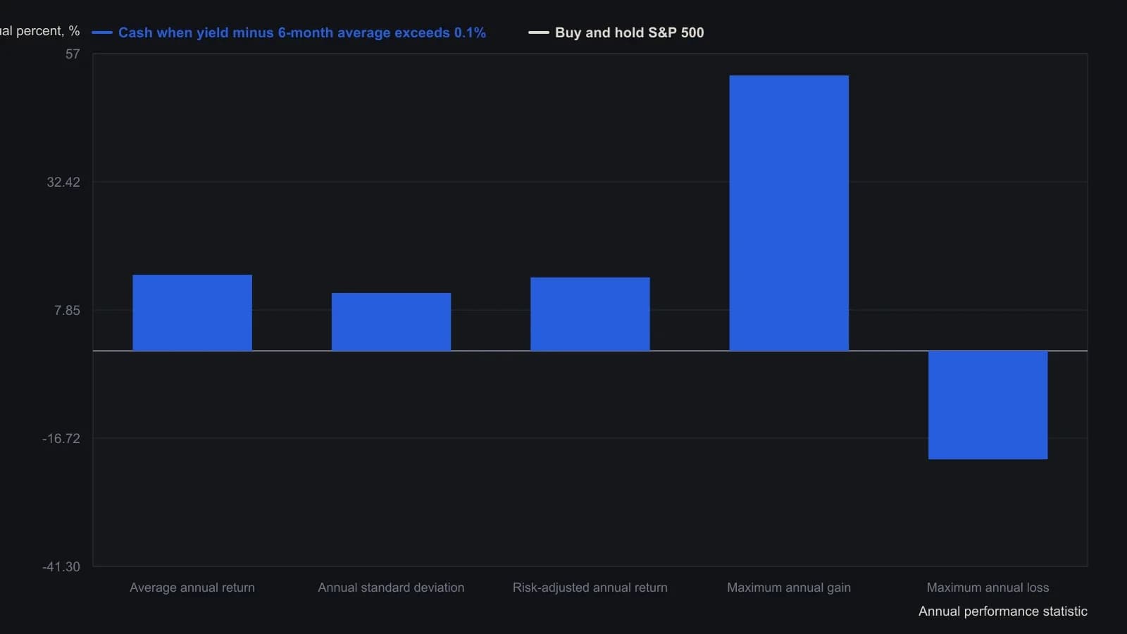
The rule uses the same month's closing yield, which the source later treated as look-ahead. Dividends are omitted. Cash earns the 90-day Treasury yield.
A split-sample linear forecast
Linear regression treated the yield-gap as the independent variable and monthly S&P 500 percentage change as the dependent variable, rather than collapsing the gap into a binary long-or-cash switch.
The split-sample-linear-fit estimated coefficients on January 1950 through December 1975 and then applied them to 1976-1995 so the predicted-monthly-change would be judged on unseen months rather than on a full-sample fit. The 1950-1975 fit was monthly S&P 500 percentage change equal to 0.859% minus 5.947 times the yield-gap, with an R-squared of 0.0591. Refitting the same inverse linear form on 1950-1995 and on 1976-1995 produced R-squared values of 0.0622 and 0.0823 respectively.
Editorial reading
Editorial reading: keeping the yield-gap continuous, fitting it on the first half of the sample, and scoring the predicted-monthly-change on the second half is the evaluation step that a binary cash switch skips. The archive R-squared values stay small across the original fit and the two refits, so the linear map is a modest association test, not a claim that the intermarket-regime-filter has been proved.
All readings on this track · 43 readings
- 1990Constructing dollar baselines from rates, inflation, and residuals
- 1990Constructing a nominal index value from forward earnings and fitted yield
- 1990Constructing a nominal index price from earnings and a fitted yield
- 1990Endpoint-pinned price paths are not forecasts
- 1990Constructing least-squares polynomial smoothers
- 1991Endpoint growth rates versus linear-regression consistency
- 1991Out-of-sample checks for linear growth fits
- 1991Trend as persistence, not a straight line
- 1991Quadratic trend, residual oscillator, and a secondary cycle calendar
- 1991Time-origin offset and residual-price divergence on a quadratic least-squares fit
- 1991A least-squares trendline from ordered prices
- 1992Constructing log-linear growth and reliability screens
- 1992Constructing log-linear growth-rate baselines
- 1992Next-session high, low, and close from rolling linear regression
- 1993Auditing an index price-earnings multiple with short-rate regression
- 1994Regression-seeded nested exponential price filter
- 1994Constructing the double exponential average from lag cancellation
- 1994Evaluating money supply as a linear leading-index baseline
- 1995Constructing least-squares trend channels
- 1995Linear baseline holdout checks for annual bill-rate forecasts
- 1995Projection bands from high and low regression slopes
- 1995Evaluating a least-squares end-point moving average on a known test series
- 1996Constructing an endpoint moving average from a least-squares line
- 1996Scoring equity path consistency with a k-ratio overlay
- 1996Evaluating month-end yield gaps for equity regimes
- 1996Constructing session-indexed standard error bands
- 1998Evaluating linear regression baselines for index valuation
- 1998R-squared as a two-state trend filter from a price-time fit
- 2000Second-order moving-average lag correction
- 2002Price regression line versus beta for index tracking
- 2003Regression slope with an r-squared trend confidence gate
- 2003Constructing finite-volume-element divergence with slope comparison
- 2004Building a daily score from regression, retracement, and volume
- 2004Constructing least-squares trendlines from ordered prices
- 2007Rectangle breakout targets beyond height
- 2007Confirming a price trend with regression slope and r-squared
- 2008A linear-regression angle assembled as one trend filter
- 2010A two-state swing machine from four running extremes
- 2016Score oil-complex tightness before divergence or regression
- 2017Nikkei-yen intermarket divergence as a regime case study
- 2017Constructing Calmar ratio and linear regression baselines
- 2019Pair-trade layer construction versus average-spread management
- 2020A convolution slope built from nested linear regression