1990issue C031-10
Constructing dollar baselines from rates, inflation, and residuals
After the dollar floated, its swings were described as transmitting into bond, equity, and gold markets. The construction task is to lock monthly-average-sampling, a lookback-compromise, and a publication-lag-offset, then treat residual-divergence against the fitted-baseline as the hypothesis.
- Lock monthly-average-sampling, the lookback-compromise, and the publication-lag-offset before ranking inputs or fitting a path.
- Same-month-correlation over 72 months from April 1983 through March 1989 ranked Japanese short-term rates first among twenty-six candidates, ahead of U.S. rates and ahead of a 0.52 merchandise-trade-deficit association.
- A same-month regression assigned a 94.5% explained-variance-share to Japanese short-term rates plus eight other series, with Japanese short-term rates contributing almost 80%; a one-month-offset mix of U.S. rates and major-economy inflation led the early-1985 and early-1988 turns.
- Residual-divergence, a flattening fitted-baseline or a widening gap versus the actual index, is the falsifiable condition; residual-autocorrelation was treated as expected because interventions sit outside the linear form.
A floating dollar as an intermarket object
After fixed exchange-rate arrangements ended in the early 1970s, the dollar floated. Its swings were described as transmitting into bond, equity, and gold markets.
Editorial reading: a dollar position is already a cross-market statement. The first job is to write an explicit linear equation, not to read the index in isolation.
Fix the window before the equation
For a longer-horizon construction, monthly averages of the dollar index and of applicable inputs were preferred over month-end prints. Consumer-price series arrive monthly, and single-day closes are more volatile. Monthly-average-sampling uses those period averages so a single volatile close does not dominate a monthly observation.
The worked construction used 72 months of monthly data from April 1983 through March 1989. That choice reflected a general practice of five-to-six-year lookbacks. The lookback-compromise is a multi-year monthly window long enough to outlast a temporary dislocation but short enough that evolving cross-market kinships are not treated as fixed.
A publication-lag-offset then shifts official rate, inflation, or flow series by one or two months relative to the dollar index so the construction uses only information that would have been in hand.
Rank drivers with same-month correlation
Twenty-six candidate series were correlated with the dollar index on a same-month basis: short- and long-term rates and consumer-price inflation for seven major economies, plus five U.S. trade and investment-flow series. Same-month-correlation is that linear association with no time offset, used to rank inputs before a regression is specified.
Over that window, Japanese short-term rates showed a same-month correlation of 0.89 with the dollar index. Japanese short- and long-term rates ranked as the two closest associations, ahead of U.S. rates. The merchandise-trade-deficit series and the dollar index had a same-month correlation of 0.52 across the 72 months, with a less negative deficit tending to coincide with a higher dollar index.
Circular flows behind the ranking
Cross-market flows were described as circular. Funds leaving Japan for the United States lifted Japanese rates and bid the dollar higher, while some of those purchases pressed U.S. Treasury yields lower, and a weaker dollar then inflicted currency losses on Japanese holders.
A same-month fitted baseline
A same-month multiple regression of the dollar index on Japanese short-term rates plus eight other inflation, yield, and U.S. overseas-investment series produced a fitted path. The coefficient of multiple determination was 94.5%, and Japanese short-term rates contributed almost 80% of the explanation.
The fitted-baseline is the monthly dollar level implied by plugging those selected cross-market inputs into a linear regression. Explained-variance-share is the portion of dollar-index variation attributed to the full regression, or to one dominant input inside that regression.
Editorial reading: a high same-month fit only shows how tightly the chosen inputs can track the index when they are allowed to sit in the same month. It is not the destination of the construction.
Offset the inputs when the baseline needs to lead
After a one-month offset to mimic data lag, a specification using U.S. rates plus inflation from seven major economies produced fitted values that led the dollar index at the early-1985 and early-1988 turns. U.S. Treasury-bond yields and Japanese inflation entered positively, and U.S. and Canadian inflation entered negatively. Rates-only inputs tracked least well as a leading baseline.
Dollar index vs one-month-offset fitted baseline
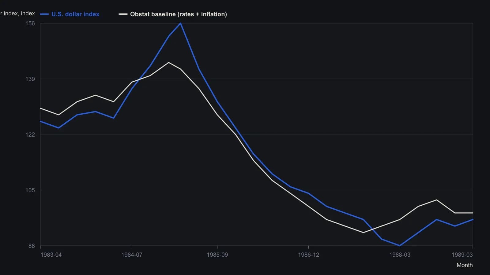
Sharp used monthly averages, a 72-month window from April 1983 to March 1989, and a one-month publication-lag offset so January inputs meet February prices. The source gave no printed coordinates; these points are approximate readings from a ratio-scale raster.
Read the residual, not a tighter fit
A five-year regression ending at the 1985 dollar peak produced fitted values whose upward slope slackened and whose gap versus the actual index widened. Residual-divergence is that flattening of the fitted baseline, or a widening gap versus the actual dollar index, treated as a falsifiable trend-change condition.
Residual-autocorrelation, the serial dependence left in regression errors, was treated as expected in market data because interventions and speculative episodes sit outside a linear specification.
All readings on this track · 43 readings
- 1990Constructing dollar baselines from rates, inflation, and residuals
- 1990Constructing a nominal index value from forward earnings and fitted yield
- 1990Constructing a nominal index price from earnings and a fitted yield
- 1990Endpoint-pinned price paths are not forecasts
- 1990Constructing least-squares polynomial smoothers
- 1991Endpoint growth rates versus linear-regression consistency
- 1991Out-of-sample checks for linear growth fits
- 1991Trend as persistence, not a straight line
- 1991Quadratic trend, residual oscillator, and a secondary cycle calendar
- 1991Time-origin offset and residual-price divergence on a quadratic least-squares fit
- 1991A least-squares trendline from ordered prices
- 1992Constructing log-linear growth and reliability screens
- 1992Constructing log-linear growth-rate baselines
- 1992Next-session high, low, and close from rolling linear regression
- 1993Auditing an index price-earnings multiple with short-rate regression
- 1994Regression-seeded nested exponential price filter
- 1994Constructing the double exponential average from lag cancellation
- 1994Evaluating money supply as a linear leading-index baseline
- 1995Constructing least-squares trend channels
- 1995Linear baseline holdout checks for annual bill-rate forecasts
- 1995Projection bands from high and low regression slopes
- 1995Evaluating a least-squares end-point moving average on a known test series
- 1996Constructing an endpoint moving average from a least-squares line
- 1996Scoring equity path consistency with a k-ratio overlay
- 1996Evaluating month-end yield gaps for equity regimes
- 1996Constructing session-indexed standard error bands
- 1998Evaluating linear regression baselines for index valuation
- 1998R-squared as a two-state trend filter from a price-time fit
- 2000Second-order moving-average lag correction
- 2002Price regression line versus beta for index tracking
- 2003Regression slope with an r-squared trend confidence gate
- 2003Constructing finite-volume-element divergence with slope comparison
- 2004Building a daily score from regression, retracement, and volume
- 2004Constructing least-squares trendlines from ordered prices
- 2007Rectangle breakout targets beyond height
- 2007Confirming a price trend with regression slope and r-squared
- 2008A linear-regression angle assembled as one trend filter
- 2010A two-state swing machine from four running extremes
- 2016Score oil-complex tightness before divergence or regression
- 2017Nikkei-yen intermarket divergence as a regime case study
- 2017Constructing Calmar ratio and linear regression baselines
- 2019Pair-trade layer construction versus average-spread management
- 2020A convolution slope built from nested linear regression