1998issue C041-3
R-squared as a two-state trend filter from a price-time fit
A market filter can classify trending and nontrending states from r-squared on a least-squares fit of closing price to time. Thresholds, optional averaging, and a run-length turn that tightness measure into a two-state gate, while slope, a linear-predicted-value, and percent-error remain secondary outputs.
- The filter squares the linear association between closing price and a time or bar-index series to obtain r-squared over a fixed lookback.
- A reading above a 0.70 trend-threshold is treated as trending; a reading below a 0.30 no-trend-threshold is treated as nontrending.
- Squared r may stay raw or be averaged, and a run-length such as 10 bars can delay a mark or alert until the state persists.
- The same fit can emit a slope, a linear-predicted-value, and a percent-error without using those series as the state gate.
How r-squared is formed
The filter begins by measuring the linear association between a closing-price series and a time or bar-index series, then squares that association to obtain r-squared. That quantity is the square of the linear association over a fixed lookback.
Several constructions use a 30-observation lookback for the price-versus-time fit. One construction uses a default correlation period of 10 rather than 30.
Trend and no-trend cutoffs
An r-squared reading above a trend-threshold of 0.70 is treated as a trending state, because price is then aligned with a straight time path. An r-squared reading below a no-trend-threshold of 0.30 is treated as a nontrending state.
SPX r-squared from a 30-bar price-time fit
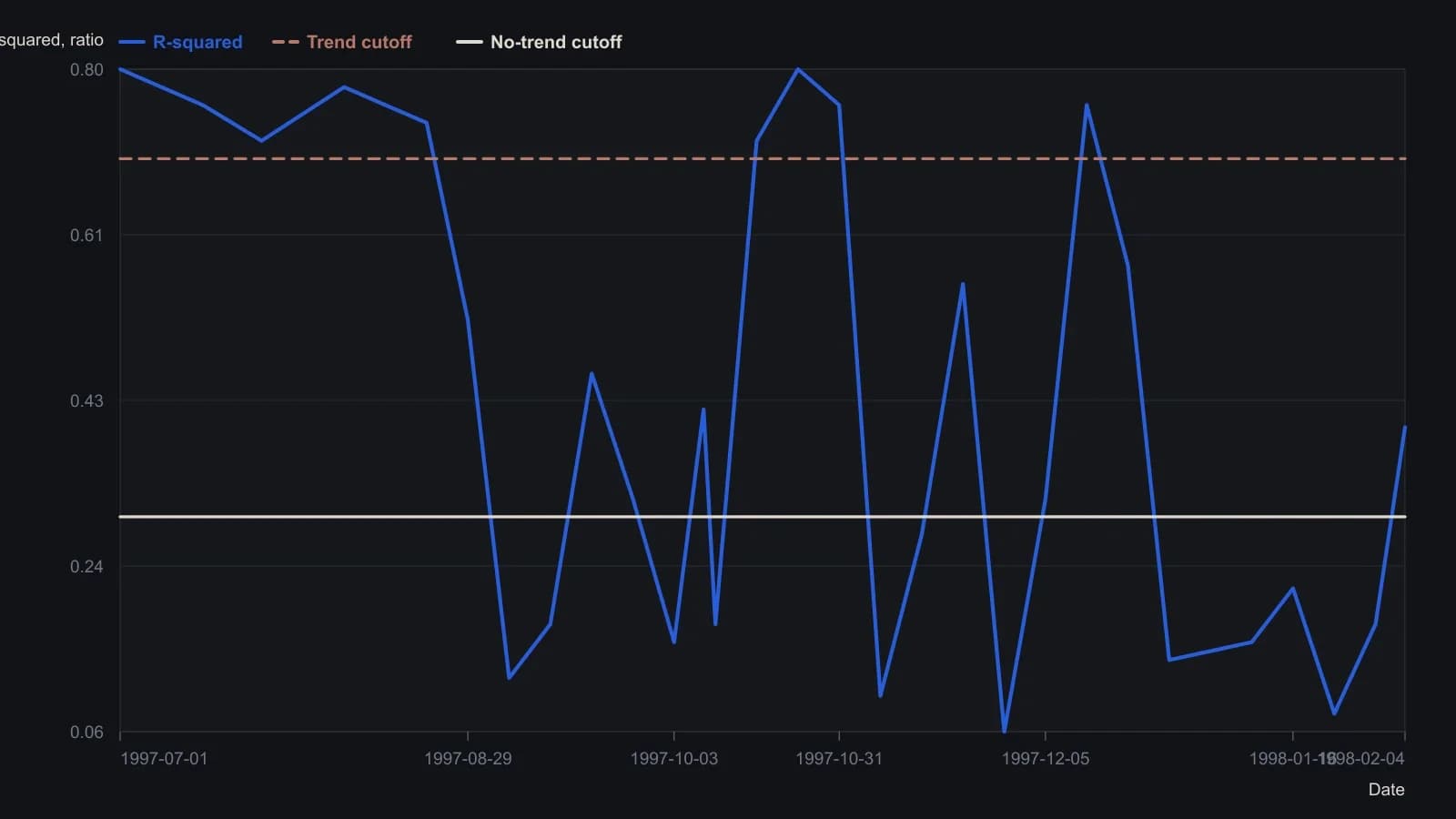
Curve digitized from the published r-squared pane, not from a table. Length is 30 bars (close versus time index). Last printed SPX print is 1006.90 on 4 Feb 1998. Approximate to about 0.02 given raster resolution; do not treat as tick-level data.
Smoothing, persistence, and painted bars
Squared r may be left raw or averaged. One construction defaults the smoother length to 1, which leaves the raw r-squared series in place.
A persistence count can require the reading to stay above or below a threshold for a stated run of bars before a mark or alert is issued. That run-length has one default of 10.
Price bars can be painted as trending or nontrending from the same r-squared series. Equal trend-threshold and no-trend-threshold inputs can force every bar into one of the two states.
Secondary outputs from the same fit
The same least-squares fit can also emit a slope, a linear-predicted-value formed from the prior close plus the prior least-squares slope, and a percent-error that expresses the close as a percentage deviation from that linear-predicted-value.
All readings on this track · 43 readings
- 1990Constructing dollar baselines from rates, inflation, and residuals
- 1990Constructing a nominal index value from forward earnings and fitted yield
- 1990Constructing a nominal index price from earnings and a fitted yield
- 1990Endpoint-pinned price paths are not forecasts
- 1990Constructing least-squares polynomial smoothers
- 1991Endpoint growth rates versus linear-regression consistency
- 1991Out-of-sample checks for linear growth fits
- 1991Trend as persistence, not a straight line
- 1991Quadratic trend, residual oscillator, and a secondary cycle calendar
- 1991Time-origin offset and residual-price divergence on a quadratic least-squares fit
- 1991A least-squares trendline from ordered prices
- 1992Constructing log-linear growth and reliability screens
- 1992Constructing log-linear growth-rate baselines
- 1992Next-session high, low, and close from rolling linear regression
- 1993Auditing an index price-earnings multiple with short-rate regression
- 1994Regression-seeded nested exponential price filter
- 1994Constructing the double exponential average from lag cancellation
- 1994Evaluating money supply as a linear leading-index baseline
- 1995Constructing least-squares trend channels
- 1995Linear baseline holdout checks for annual bill-rate forecasts
- 1995Projection bands from high and low regression slopes
- 1995Evaluating a least-squares end-point moving average on a known test series
- 1996Constructing an endpoint moving average from a least-squares line
- 1996Scoring equity path consistency with a k-ratio overlay
- 1996Evaluating month-end yield gaps for equity regimes
- 1996Constructing session-indexed standard error bands
- 1998Evaluating linear regression baselines for index valuation
- 1998R-squared as a two-state trend filter from a price-time fit
- 2000Second-order moving-average lag correction
- 2002Price regression line versus beta for index tracking
- 2003Regression slope with an r-squared trend confidence gate
- 2003Constructing finite-volume-element divergence with slope comparison
- 2004Building a daily score from regression, retracement, and volume
- 2004Constructing least-squares trendlines from ordered prices
- 2007Rectangle breakout targets beyond height
- 2007Confirming a price trend with regression slope and r-squared
- 2008A linear-regression angle assembled as one trend filter
- 2010A two-state swing machine from four running extremes
- 2016Score oil-complex tightness before divergence or regression
- 2017Nikkei-yen intermarket divergence as a regime case study
- 2017Constructing Calmar ratio and linear regression baselines
- 2019Pair-trade layer construction versus average-spread management
- 2020A convolution slope built from nested linear regression