2020issue C0150-56
A convolution slope built from nested linear regression
A slope series can be rebuilt by nesting a one-bar-ahead linear-regression projection inside a second, shorter regression. The second lookback is taken from the first window, which keeps the same indicator family consistent across platforms.
- The projection step is a linear-regression value of the chosen price series over a user length, evaluated one bar ahead.
- The convolution length is the integer portion of the square root of that first lookback, not a separately chosen window.
- The plotted slope is the linear-regression slope of the projection series over the same shortened length.
- Platform listings add an unsure band, an acceleration series, and experimental entry and exit tests, but they do not complete a full rule set.
What the nested pair is doing
This archive article shows how a slope series is built by nesting one linear-regression step inside another. The first step produces a one-bar-ahead projection of the chosen price series. The second step fits a shorter linear regression to that projection series.
How the projection is formed
The projection step, called leavitt-projection in this article, is defined as a linear-regression value of the chosen price series over a user length, evaluated one bar ahead. Linear-regression here means a fitted line through an ordered lookback of prices that yields a projected next value and a slope.
How the shortened lookback is chosen
The second lookback is not a separately chosen window. The convolution length is the integer portion of the square root of the first lookback. In this construction that shorter lookback is the moving-average window applied to the projection series.
The convolution series and the plotted slope
The convolution series, called leavitt-convolution here, is a second linear-regression value of the projection series over that shortened length, again evaluated one bar ahead. The plotted slope series, called leavitt-convolution-slope, is the linear-regression slope of the projection series over the same shortened length.
How one listing draws the slope
A published TradeStation listing uses close as the default price, a length of 61, and an unsure band of 0.2. The unsure-band is a small symmetric threshold around zero used only to shade an indecisive zone on the slope plot. That listing colors the slope histogram by whether the latest reading is above or below the prior bar.
Where the same construction appears
The same construction is shown as a chart study on a 15-minute equity-index futures contract, a daily equity, and a 30-minute energy futures contract.
Experimental rules and the acceleration companion
One platform listing notes that the source article does not supply complete system rules. That listing then defines an experimental long entry when both the convolution slope and its one-bar change are above zero. The same experimental exit waits until the convolution slope makes a 20-bar high and the one-bar change in slope then turns negative. A one-bar difference of the convolution slope is plotted as a companion acceleration series, called lc-acceleration in this article, in at least one vendor listing. That companion is used as a sign-change detector.
Later listings of the projection and convolution pair
Two later listings plot the projection and convolution pair on the same broad-market fund with a 100-bar first length. In one of those environments the two studies are required to live in separate files.
Leavitt projection and convolution on SPY
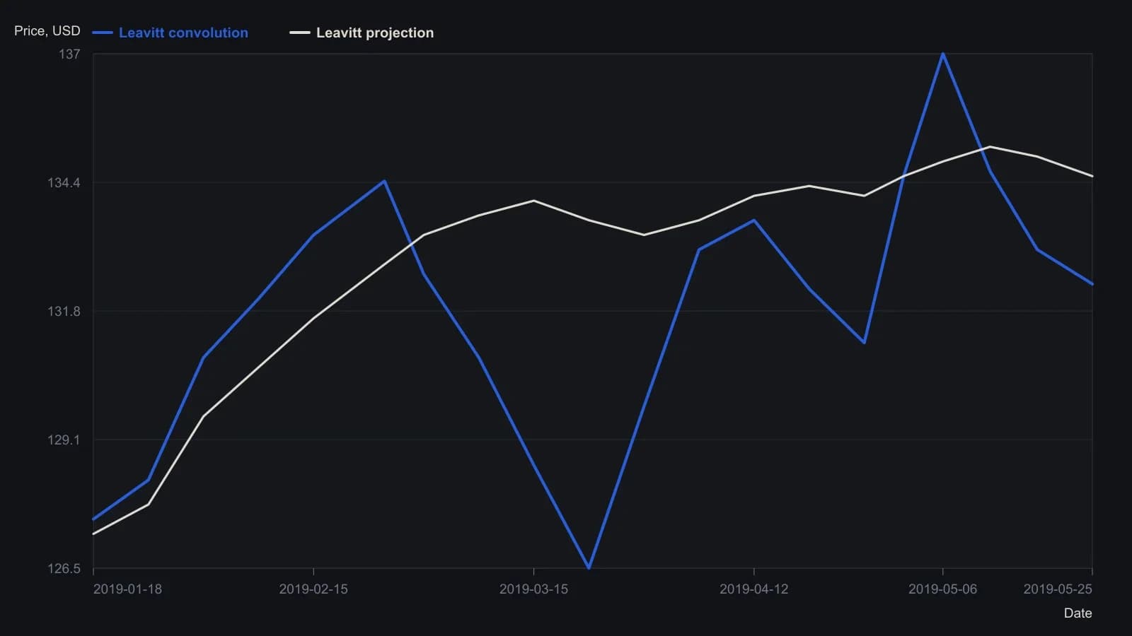
Figure 9 fixes length at 100 bars, so the convolution window is floor(sqrt(100)) = 10. The figure labels months February–May and does not print a year or session interval; y-values are approximate raster readings.
All readings on this track · 43 readings
- 1990Constructing dollar baselines from rates, inflation, and residuals
- 1990Constructing a nominal index value from forward earnings and fitted yield
- 1990Constructing a nominal index price from earnings and a fitted yield
- 1990Endpoint-pinned price paths are not forecasts
- 1990Constructing least-squares polynomial smoothers
- 1991Endpoint growth rates versus linear-regression consistency
- 1991Out-of-sample checks for linear growth fits
- 1991Trend as persistence, not a straight line
- 1991Quadratic trend, residual oscillator, and a secondary cycle calendar
- 1991Time-origin offset and residual-price divergence on a quadratic least-squares fit
- 1991A least-squares trendline from ordered prices
- 1992Constructing log-linear growth and reliability screens
- 1992Constructing log-linear growth-rate baselines
- 1992Next-session high, low, and close from rolling linear regression
- 1993Auditing an index price-earnings multiple with short-rate regression
- 1994Regression-seeded nested exponential price filter
- 1994Constructing the double exponential average from lag cancellation
- 1994Evaluating money supply as a linear leading-index baseline
- 1995Constructing least-squares trend channels
- 1995Linear baseline holdout checks for annual bill-rate forecasts
- 1995Projection bands from high and low regression slopes
- 1995Evaluating a least-squares end-point moving average on a known test series
- 1996Constructing an endpoint moving average from a least-squares line
- 1996Scoring equity path consistency with a k-ratio overlay
- 1996Evaluating month-end yield gaps for equity regimes
- 1996Constructing session-indexed standard error bands
- 1998Evaluating linear regression baselines for index valuation
- 1998R-squared as a two-state trend filter from a price-time fit
- 2000Second-order moving-average lag correction
- 2002Price regression line versus beta for index tracking
- 2003Regression slope with an r-squared trend confidence gate
- 2003Constructing finite-volume-element divergence with slope comparison
- 2004Building a daily score from regression, retracement, and volume
- 2004Constructing least-squares trendlines from ordered prices
- 2007Rectangle breakout targets beyond height
- 2007Confirming a price trend with regression slope and r-squared
- 2008A linear-regression angle assembled as one trend filter
- 2010A two-state swing machine from four running extremes
- 2016Score oil-complex tightness before divergence or regression
- 2017Nikkei-yen intermarket divergence as a regime case study
- 2017Constructing Calmar ratio and linear regression baselines
- 2019Pair-trade layer construction versus average-spread management
- 2020A convolution slope built from nested linear regression