1995issue C021-8
Constructing least-squares trend channels
A trend channel can be built in three parts: a least-squares centerline on a window of closes, parallel bounds set by residual-spread, and a shared-price-scale so the fitted geometry can be checked on the same bars that built it.
- A linear-regression fit through a window of closes returns one fitted value for each observation and supplies the trendline centerline.
- Residual-spread is the population standard deviation of close minus fitted value on that same window, and it places parallel bounds two residual standard deviations above and below the centerline.
- High-low-close-structure occupies the first price-axis group, while the fitted line and bands occupy a later overlay group that must use the same vertical range.
- Dating the construction window on the category axis keeps the fitted line and bands aligned with the observation order used in the regression.
Three parts on the same bars
The construction treats a trendline as three parts that stay on the same bars: a centerline from linear-regression, parallel bounds from residual-spread, and a shared-price-scale that lets the fitted geometry be read against price.
A straight centerline through a window of closes can be produced with a least-squares fit that returns one fitted value for each observation in that window.
Fit the centerline with linear-regression
Linear-regression is a least-squares fit to an ordered window of closes. It supplies an explicit centerline baseline for the channel by returning one fitted value for each observation in that window.
Place bounds from residual-spread
Residual-spread is the dispersion of close minus fitted value over the same window used for the fit. Residual width is the population standard deviation of that difference, computed over the same observations used for the fit.
Parallel channel bounds can be placed two residual standard deviations above and below that centerline.
S&P 500 least-squares trend channel, Jan–May 1994
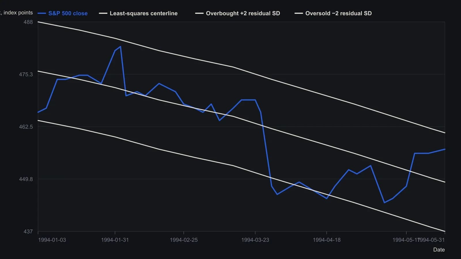
Excel TREND on closes D2:D104 for 3 Jan–31 May 1994; bands are E±2·STDEVP(close−trend). Digitized from the raster, so prices are approximate to about one index point and the series is thinned to stay within 60 points.
Plot high-low-close-structure on a shared-price-scale
High-low-close-structure is the first plotted series group: highs, lows, and closes rendered as bars so the fitted geometry is read against actual price range, not against a line sketch of closes alone.
High, low, and close can occupy that first group on the price axis, while the fitted line and its offset bands occupy a later overlay group. Connecting strokes on the high and low series can be suppressed so the first group reads as high-low bars, with a distinct close mark on each bar.
Shared-price-scale is the rule that the overlay axis holding the fitted line and bands must use the same range as the high-low-close axis so the channel is not optically distorted. Splitting later series onto an overlay axis is required whenever those series live on a different numeric range than price, including a bounded oscillator.
Keep the window in observation order
The construction window can be dated on the category axis so the fitted line and bands stay aligned with the same observation order used in the regression.
Editorial reading
Editorial: the finished channel is read here as a trendline, a constructed centerline and offset bounds that later bars can confirm or break. That sentence is a TradersWeek interpretation of the historical workflow and is not an archive claim.
All readings on this track · 43 readings
- 1990Constructing dollar baselines from rates, inflation, and residuals
- 1990Constructing a nominal index value from forward earnings and fitted yield
- 1990Constructing a nominal index price from earnings and a fitted yield
- 1990Endpoint-pinned price paths are not forecasts
- 1990Constructing least-squares polynomial smoothers
- 1991Endpoint growth rates versus linear-regression consistency
- 1991Out-of-sample checks for linear growth fits
- 1991Trend as persistence, not a straight line
- 1991Quadratic trend, residual oscillator, and a secondary cycle calendar
- 1991Time-origin offset and residual-price divergence on a quadratic least-squares fit
- 1991A least-squares trendline from ordered prices
- 1992Constructing log-linear growth and reliability screens
- 1992Constructing log-linear growth-rate baselines
- 1992Next-session high, low, and close from rolling linear regression
- 1993Auditing an index price-earnings multiple with short-rate regression
- 1994Regression-seeded nested exponential price filter
- 1994Constructing the double exponential average from lag cancellation
- 1994Evaluating money supply as a linear leading-index baseline
- 1995Constructing least-squares trend channels
- 1995Linear baseline holdout checks for annual bill-rate forecasts
- 1995Projection bands from high and low regression slopes
- 1995Evaluating a least-squares end-point moving average on a known test series
- 1996Constructing an endpoint moving average from a least-squares line
- 1996Scoring equity path consistency with a k-ratio overlay
- 1996Evaluating month-end yield gaps for equity regimes
- 1996Constructing session-indexed standard error bands
- 1998Evaluating linear regression baselines for index valuation
- 1998R-squared as a two-state trend filter from a price-time fit
- 2000Second-order moving-average lag correction
- 2002Price regression line versus beta for index tracking
- 2003Regression slope with an r-squared trend confidence gate
- 2003Constructing finite-volume-element divergence with slope comparison
- 2004Building a daily score from regression, retracement, and volume
- 2004Constructing least-squares trendlines from ordered prices
- 2007Rectangle breakout targets beyond height
- 2007Confirming a price trend with regression slope and r-squared
- 2008A linear-regression angle assembled as one trend filter
- 2010A two-state swing machine from four running extremes
- 2016Score oil-complex tightness before divergence or regression
- 2017Nikkei-yen intermarket divergence as a regime case study
- 2017Constructing Calmar ratio and linear regression baselines
- 2019Pair-trade layer construction versus average-spread management
- 2020A convolution slope built from nested linear regression