1996issue C091
Constructing session-indexed standard error bands
A 21-observation linear regression of closes on a session index supplies a local trend level and a residual width. After both series are smoothed, they form a standard-error band, and a band-location reading is taken only once that shared clock is in place.
- Use a session index as the independent variable so each bar advances the clock by one unit and non-trading days do not widen the spacing.
- Estimate the latest fitted level and the residual standard error on the same 21-observation window of closes, then smooth both with a three-period simple moving average.
- Place the upper and lower envelopes a distance of twice the smoothed residual standard error from the smoothed fitted level.
- Map the close onto the interval between those envelopes only after both series exist, and keep the smoothed coefficient of determination and the slope as tightness and direction companions.
Three series on one clock
A standard-error band is assembled from closing prices and a session index. Linear regression fits those ordered closes to the session index over a fixed lookback. The latest fitted value is the local trend level. The same lookback also yields residual width, a slope, and tightness of fit.
A short simple moving average is applied to the latest fitted level, the residual-width series, and the tightness-of-fit series. Each published value then changes more slowly than the raw statistic.
Why the independent variable is a session index
The independent variable is a running integer index rather than calendar dates. The session index assigns a consecutive integer to each trading observation so the independent variable advances one unit per bar instead of by calendar spacing. Non-trading days do not widen the x-spacing.
Session-indexed close with two-standard-error bands
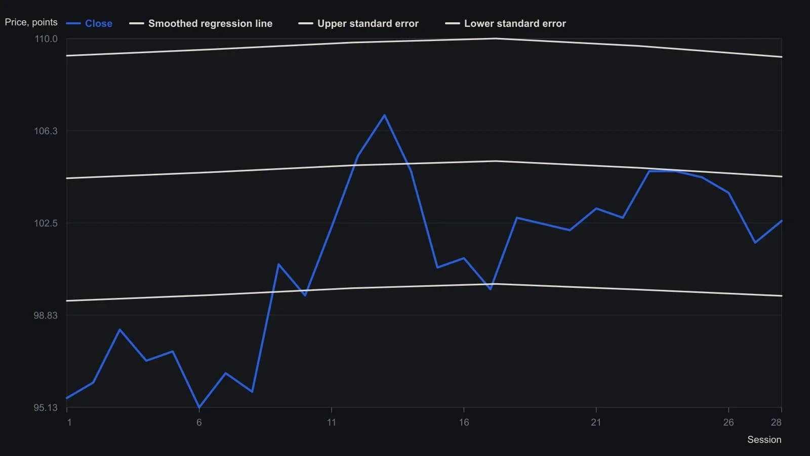
Regression and band columns stay blank until the lookback is full: raw regression level and standard error begin on session 21; the smoothed line and the two plotted bands begin on session 23.
One window for the centerline and the residual width
A 21-observation linear regression of closing prices supplies the latest fitted value as the local trend level. The residual standard error is estimated over the same 21-observation window of closes and integer index values.
Smooth both series, then place the envelopes
Both the latest fitted level and the residual-standard-error series are then smoothed with a three-period simple moving average. The upper envelope equals the smoothed fitted level plus twice the smoothed residual standard error. The lower envelope subtracts that same quantity. Those envelopes are the standard-error band: a pair placed a fixed multiple of the smoothed residual error above and below the smoothed fitted level.
The location reading after both series exist
A band-location reading maps the close onto the interval between the lower and upper envelopes. The reading exceeds 100 when the close is above the upper envelope and falls below 0 when the close is beneath the lower envelope.
Editorial note: the location reading is a rescaling of the close onto that interval. It is not available until the centerline and the residual-width series already share the session index.
Tightness of fit beside the band
The coefficient of determination is the squared correlation of closes with the integer index over the 21-observation window. That coefficient of determination is itself smoothed with a three-period simple moving average. A companion slope is taken from a linear estimate of closes against the same integer index.
All readings on this track · 43 readings
- 1990Constructing dollar baselines from rates, inflation, and residuals
- 1990Constructing a nominal index value from forward earnings and fitted yield
- 1990Constructing a nominal index price from earnings and a fitted yield
- 1990Endpoint-pinned price paths are not forecasts
- 1990Constructing least-squares polynomial smoothers
- 1991Endpoint growth rates versus linear-regression consistency
- 1991Out-of-sample checks for linear growth fits
- 1991Trend as persistence, not a straight line
- 1991Quadratic trend, residual oscillator, and a secondary cycle calendar
- 1991Time-origin offset and residual-price divergence on a quadratic least-squares fit
- 1991A least-squares trendline from ordered prices
- 1992Constructing log-linear growth and reliability screens
- 1992Constructing log-linear growth-rate baselines
- 1992Next-session high, low, and close from rolling linear regression
- 1993Auditing an index price-earnings multiple with short-rate regression
- 1994Regression-seeded nested exponential price filter
- 1994Constructing the double exponential average from lag cancellation
- 1994Evaluating money supply as a linear leading-index baseline
- 1995Constructing least-squares trend channels
- 1995Linear baseline holdout checks for annual bill-rate forecasts
- 1995Projection bands from high and low regression slopes
- 1995Evaluating a least-squares end-point moving average on a known test series
- 1996Constructing an endpoint moving average from a least-squares line
- 1996Scoring equity path consistency with a k-ratio overlay
- 1996Evaluating month-end yield gaps for equity regimes
- 1996Constructing session-indexed standard error bands
- 1998Evaluating linear regression baselines for index valuation
- 1998R-squared as a two-state trend filter from a price-time fit
- 2000Second-order moving-average lag correction
- 2002Price regression line versus beta for index tracking
- 2003Regression slope with an r-squared trend confidence gate
- 2003Constructing finite-volume-element divergence with slope comparison
- 2004Building a daily score from regression, retracement, and volume
- 2004Constructing least-squares trendlines from ordered prices
- 2007Rectangle breakout targets beyond height
- 2007Confirming a price trend with regression slope and r-squared
- 2008A linear-regression angle assembled as one trend filter
- 2010A two-state swing machine from four running extremes
- 2016Score oil-complex tightness before divergence or regression
- 2017Nikkei-yen intermarket divergence as a regime case study
- 2017Constructing Calmar ratio and linear regression baselines
- 2019Pair-trade layer construction versus average-spread management
- 2020A convolution slope built from nested linear regression