2016issue C028-9
Score oil-complex tightness before divergence or regression
An oil-linked currency complex is ranked in a correlation matrix before a method is chosen. Tight coupling points to band-based divergence, a dominant driver points to single-variable regression, and a second regressor is withheld unless it is only weakly related to the first.
- Rank the Canadian dollar, a large domestic producer, an oil-service basket, and crude in a correlation matrix before assigning divergence or regression.
- In a 2005 to 2015 sample the currency tracked crude more closely than it tracked the producer or the service basket, while the producer and the basket showed tight coupling and few distinct divergence setups.
- High-price decoupling can break the usual currency-oil mapping after crude has already printed an extreme, and a later producer-basket split may be name-specific decoupling rather than a temporary market inefficiency.
- Keep single-variable regression for a dominant driver, withhold multiple regression when the extra driver is already aligned with the first, and use band-based divergence on tightly correlated legs.
Start with the oil-linked currency complex
An oil-linked currency complex is a four-market set used to place one currency trade in context: the Canadian dollar, a large domestic producer, an oil-service basket, and crude.
A correlation matrix is a table of pairwise sample correlations that ranks which legs of the complex actually move together before a model is chosen.
What the sample matrix ranked first
In a 2005 to 2015 sample, the Canadian dollar's correlation with crude oil was 0.81, higher than its correlation with a large Canadian producer (0.54) or an oil-service basket (0.53).
In that same matrix the producer correlated more strongly with crude oil (0.62) than with the Canadian dollar (0.54).
Tight coupling leaves few divergence setups
The producer and the oil-service basket printed a 0.93 pairwise correlation and, on a weekly overlay with crude, tended to travel together, leaving fewer distinct divergence setups.
Tight coupling is a very high pairwise correlation that leaves few lasting separations for a divergence rule.
Weekly Suncor, oil-service ETF, and crude
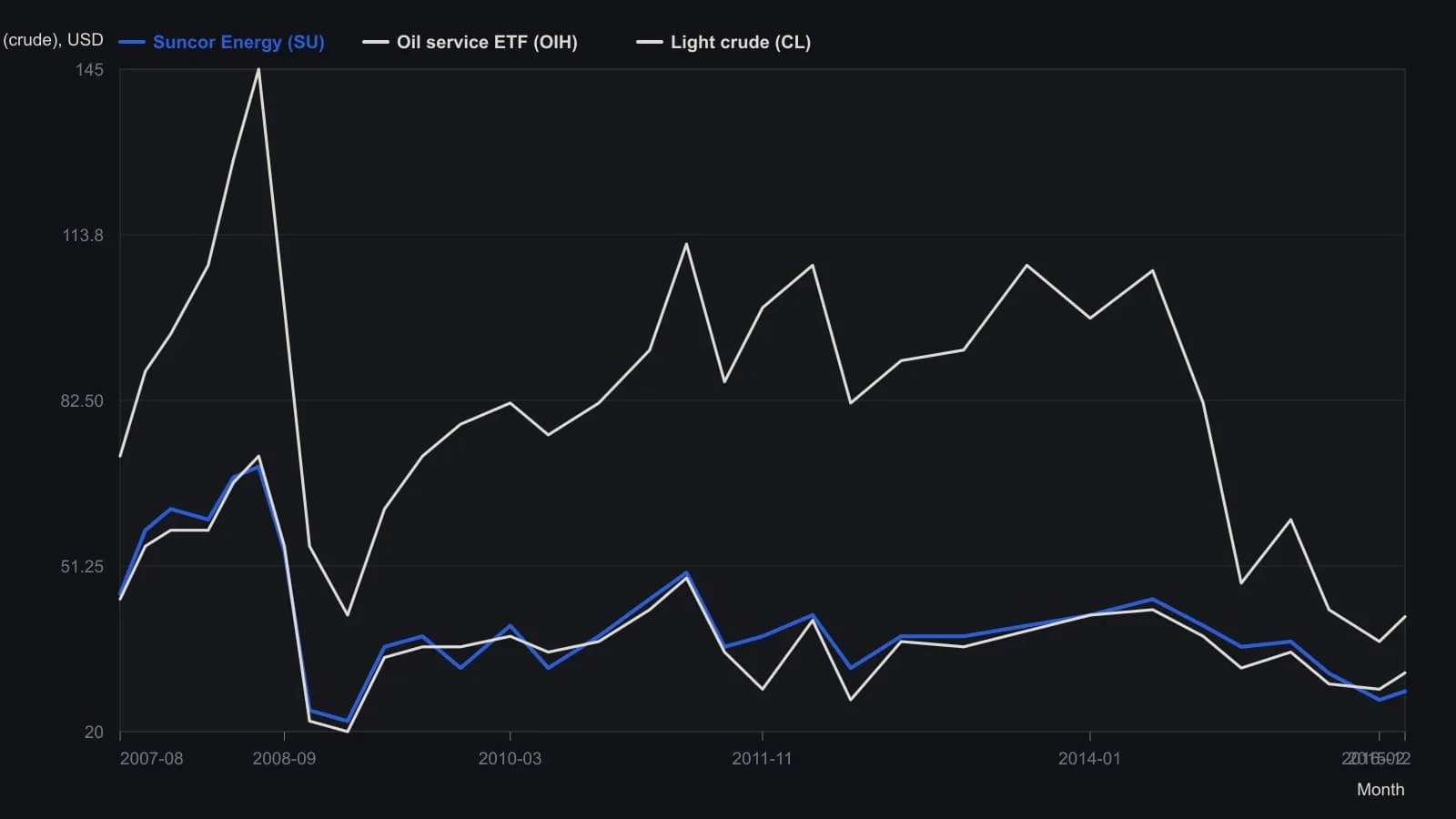
Suncor and OIH are dollars per share on the source right scale; light crude is dollars per barrel on the left scale. Interior points are digitized from a weekly raster and are approximate.
High-price decoupling can break the currency-oil map
The currency-oil mapping was described as able to break down at very high crude prices. In 2008, with oil near 140, the Canadian dollar peaked almost eight months earlier. In 2011, with oil near 110, the currency formed a double top before following oil lower.
High-price decoupling is a regime in which the usual Canadian-dollar and crude mapping weakens after oil has already printed an extreme.
A price comparison of the producer, crude, and the Canadian dollar showed the producer turning down before crude in 2008 and later diverging. In 2011 both crude and the producer diverged versus the currency.
Tight coupling and name-specific decoupling
When a producer and its sector basket are that tightly coupled, a later split cannot be confidently read as a temporary market inefficiency rather than a name-specific problem.
Name-specific decoupling is a split between a producer and its sector basket that may reflect a company event rather than a temporary market inefficiency.
When regression gives way to band-based divergence
A single-variable linear regression was the first design tried for a Canadian-dollar system and was then replaced with a band-based divergence method after the regression was judged inadequate.
Single-variable regression is a linear forecast that maps one intermarket driver onto a target over a defined lookback. Band-based divergence is a price-indicator condition that flags even small separations between related markets and is used when those markets are tightly correlated.
Band-based divergence was argued to suit tightly correlated markets because it can register small separations and therefore produce more signals, whereas multiple regression was said to add value only when the independent variables themselves are weakly correlated.
A regression of the producer on the oil-service basket did not raise r-squared when crude was added as a second independent variable, and substituting the Canadian dollar for crude improved the fit only slightly. Multiple regression is a linear forecast that adds a second driver only when that driver is not already highly collinear with the first.
Editorial reading of the workflow
Editorial reading: the sample matrix made crude the dominant Canadian-dollar driver, so a single-variable map from crude to the currency was the first quantitative design. The producer-basket pair was too tightly coupled for a second crude regressor to lift the fit, and substituting the Canadian dollar helped only slightly.
Editorial reading: band-based divergence is assigned to tightly correlated legs that can still print small separations, not to a later producer-basket split that cannot be separated from name-specific decoupling. High-price decoupling is a reminder that even the tightest currency-oil rank can weaken after crude has already printed an extreme.
All readings on this track · 43 readings
- 1990Constructing dollar baselines from rates, inflation, and residuals
- 1990Constructing a nominal index value from forward earnings and fitted yield
- 1990Constructing a nominal index price from earnings and a fitted yield
- 1990Endpoint-pinned price paths are not forecasts
- 1990Constructing least-squares polynomial smoothers
- 1991Endpoint growth rates versus linear-regression consistency
- 1991Out-of-sample checks for linear growth fits
- 1991Trend as persistence, not a straight line
- 1991Quadratic trend, residual oscillator, and a secondary cycle calendar
- 1991Time-origin offset and residual-price divergence on a quadratic least-squares fit
- 1991A least-squares trendline from ordered prices
- 1992Constructing log-linear growth and reliability screens
- 1992Constructing log-linear growth-rate baselines
- 1992Next-session high, low, and close from rolling linear regression
- 1993Auditing an index price-earnings multiple with short-rate regression
- 1994Regression-seeded nested exponential price filter
- 1994Constructing the double exponential average from lag cancellation
- 1994Evaluating money supply as a linear leading-index baseline
- 1995Constructing least-squares trend channels
- 1995Linear baseline holdout checks for annual bill-rate forecasts
- 1995Projection bands from high and low regression slopes
- 1995Evaluating a least-squares end-point moving average on a known test series
- 1996Constructing an endpoint moving average from a least-squares line
- 1996Scoring equity path consistency with a k-ratio overlay
- 1996Evaluating month-end yield gaps for equity regimes
- 1996Constructing session-indexed standard error bands
- 1998Evaluating linear regression baselines for index valuation
- 1998R-squared as a two-state trend filter from a price-time fit
- 2000Second-order moving-average lag correction
- 2002Price regression line versus beta for index tracking
- 2003Regression slope with an r-squared trend confidence gate
- 2003Constructing finite-volume-element divergence with slope comparison
- 2004Building a daily score from regression, retracement, and volume
- 2004Constructing least-squares trendlines from ordered prices
- 2007Rectangle breakout targets beyond height
- 2007Confirming a price trend with regression slope and r-squared
- 2008A linear-regression angle assembled as one trend filter
- 2010A two-state swing machine from four running extremes
- 2016Score oil-complex tightness before divergence or regression
- 2017Nikkei-yen intermarket divergence as a regime case study
- 2017Constructing Calmar ratio and linear regression baselines
- 2019Pair-trade layer construction versus average-spread management
- 2020A convolution slope built from nested linear regression