1990issue C071-2
Build a weekly leading sector composite from scaled transports and financials
A leading sector composite is assembled by scaling weekly closes of a transportation average with bank, insurance, and financial indices, then averaging them. Editorial reading: plot that finished series against an equity benchmark so a later high-low split can be treated as a regime check on a single stock or index idea, not as a standalone forecast.
- Assemble the leading sector composite from four listed equity-group series: a transportation average, a bank index, an insurance index, and a financial index.
- Those four series were selected because they appeared to lead the broader equity market over an intermediate horizon of eight weeks.
- Use weekly construction and equal-weight scaling: divide the transportation close by three, triple the financial-index close, leave the bank and insurance closes unscaled, then average the four adjusted values.
- Plot the finished series against a chosen equity benchmark. In October 1989 the composite formed lower highs while the industrial average formed higher highs, a split treated as a cautionary divergence, and further historical testing was still described as needed.
Four series in one composite
The leading sector composite is a single series formed by scaling and averaging a transportation average with bank, insurance, and financial indices. Those four listed equity-group series were selected because they appeared to lead the broader equity market over an intermediate horizon defined as eight weeks.
Weekly scaling before the average
The same construction can be run on daily or weekly closes. The documented example uses weekly construction, computing the composite from weekly closing levels rather than from daily prints.
Each weekly close is scaled before averaging. Equal-weight scaling divides the transportation series by three, multiplies the financial series by three, and leaves the bank and insurance series unscaled so no single leg dominates. The four adjusted values are then averaged.
Compare the composite with a benchmark
The finished series is plotted against a chosen equity benchmark so the two paths can be compared on the same chart. A benchmark split is a chart condition in which the composite and a tracked equity average print opposite sequences of highs or lows.
One comparison chart covers 65 weeks and ends on 9 March 1990. In October 1989 the composite formed lower highs while the industrial average formed higher highs, a split treated as a cautionary divergence.
Companion views still to test
Further historical testing was described as still needed. Point-and-figure charting and 20-, 50-, and 200-day moving averages were proposed as companion views.
Weekly DJIA versus the mixture index, Dec 1988–Mar 1990
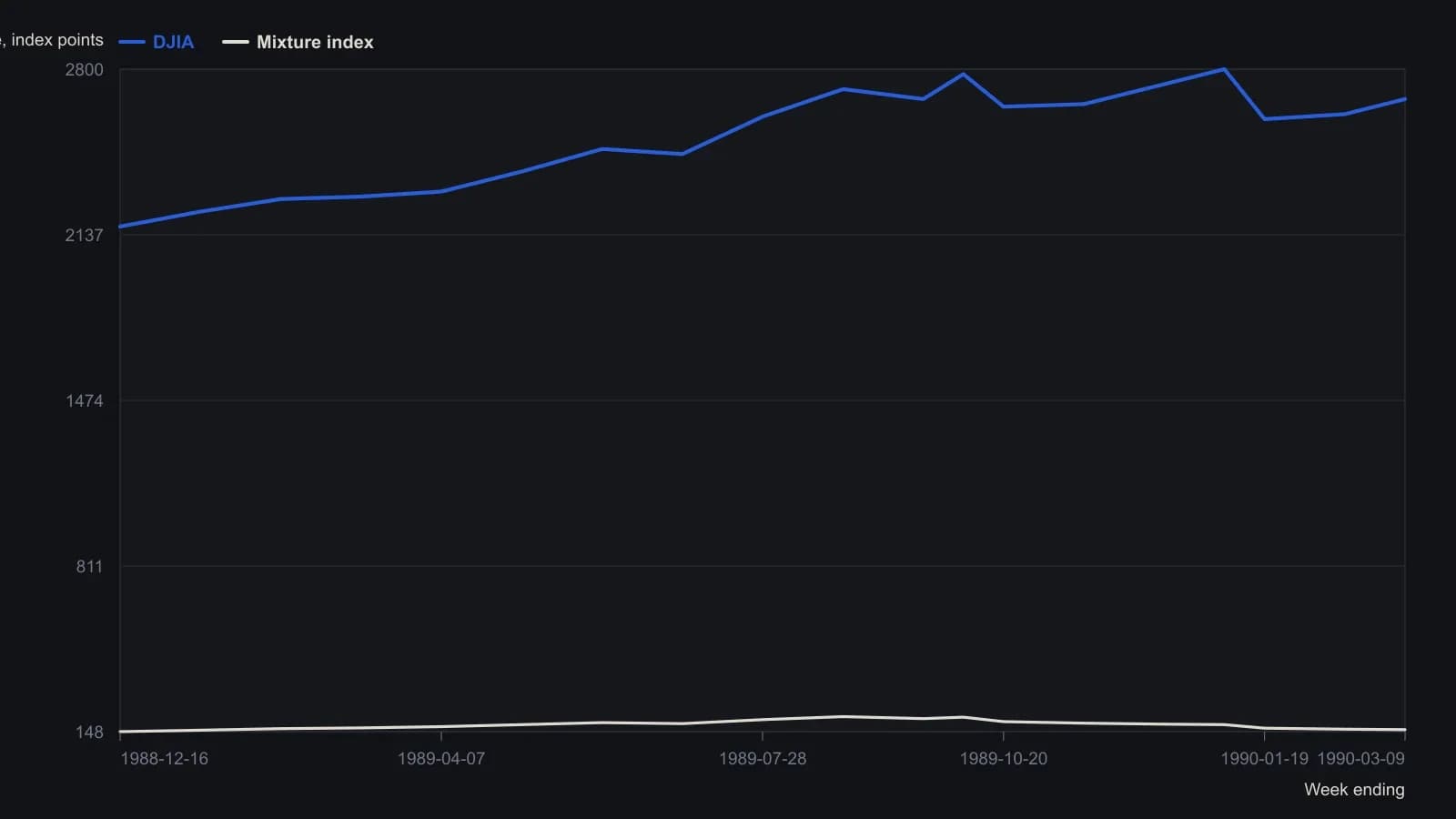
Axis numerals on the scan are degraded and the frame is inverted relative to a conventional high-at-top plot; y-values are approximate weekly closes taken from the printed scales (Dow at 200-point steps, mixture at 20-point steps) after restoring that orientation. No source table was printed.
All readings on this track · 32 readings
- 1989Volume confirmation windows and exponential average construction
- 1990Constructing stochastic %K and %D from range position
- 1990Build a weekly leading sector composite from scaled transports and financials
- 1990Constructing stochastic K and D lines and divergence cues
- 1993Relative strength index events depend on the chosen input combination
- 1995Constructing a dual-horizon force index
- 1996Building a range-normalized divergence index from relative strength index
- 1998Treat RSI as a testable filter rather than a trigger
- 1999Primary-cycle windows, then stochastic confirmation
- 1999Stochastic rules versus buy and hold
- 2001Constructing confirmation filters for RSI overbought and oversold extremes
- 2003Constructing divergence-equivalent relative strength index and stochastic oscillators
- 2003Reverse-engineered RSI as a next-close projection
- 2003Scoring open versus resolved relative strength divergences
- 2003Bull-and-bear-balance from OHLC bar patterns
- 2003Constructing bull and bear balance from session paths
- 2004Four-month rule: auto stocks as a market-regime warning
- 2004Constructing stochastic oscillator bands, crosses and divergence
- 2004Volume as an independent check on price oscillators
- 2004Simple dual confirmation for a short-horizon index-futures system
- 2005Confirm a stochastic divergence by reclaiming the first-swing bar
- 2005Weekly stochastic divergence and a long average on 2005 high-yield entrants
- 2005Predicted averages from related market baskets
- 2006Rank price-oscillator divergences, then filter by trend
- 2006Relative-spread-strength for cycle confirmation
- 2007Weekly breakout stretch and histogram divergence
- 2011A luxury-auction stock as a cross-market bubble warning
- 2014Running-percentile close divergences and trend filters
- 2015Rebuilding the relative strength index from close-to-average gaps
- 2016Constructing higher-high and lower-low stochastic pairs
- 2018Constructing composite relative-strength-index stochastics for reversal confirmation
- 2019Building a smoothed Stochastic oscillator of the Relative Strength Index for Price-indicator divergence checks