1990issue C041-10
Two clocks for copper: a factor regime, a regression baseline, and leftover moving-average timing
A historical copper workflow scored monthly drivers, fitted an explicit linear path on that same clock, and reserved a short nearest-contract moving average for leftover timing. Editorial reading: build the weeks-to-months regime and the explained level first, then let the daily average answer only the state those models cannot resolve.
- Monthly averages were the regime clock: copper was paired with inflation, rates, the dollar, and inventories and scored from exact inverse through no measured link to exact match.
- Same-month linear regression attributed about 92 percent of monthly-average variance to the Consumer Price Index, Treasury bill rates, and selected rates of change, with the CPI level alone about 85 percent. A one-month-off-shift of consumer and producer prices was the workable late print.
- The fitted statistical path was compared with actual monthly averages to mark leading turns and stretches, using a Durbin-Watson check and leaving room for unquantified shocks.
- A 13-day moving average of nearest-contract closes set a long-or-cash state from the prior close, and a 1.05 multiple of a six-day average marked a short-horizon stretch treated as ready for a correction.
Two clocks on one metal
The archive copper workflow used two sampling clocks rather than one blended score. Correlation analysis ranked how tightly monthly-average copper moved with candidate drivers. Linear regression then attributed a share of that monthly-average variance to a short list of series and produced a fitted statistical path.
A moving average of nearest-contract closes was kept for a separate question: whether the prior close sat above or below a short simple average.
Monthly pairings as a regime map
Correlation analysis paired copper with candidate drivers on monthly averages, the sampling interval presented as the usual balance between short-term volatility and timely information. Each pair received a score from +1 through 0 to -1, a pairwise reading from exact match through no measured link to exact inverse.
On 50 months through May 1989, monthly copper showed a 0.93 correlation with the Consumer Price Index, a 0.06 correlation with Treasury bond yields, and a -0.6 correlation with the U.S. dollar index. U.S. refined copper stocks had a monthly correlation of -0.81 with copper, a weaker absolute reading than the CPI pairing, even though inventory and delivery statistics were the more commonly discussed supply-demand inputs.
A daily pairing window
Over a 100-day daily window, copper prices showed a high correlation with gold and a stronger link to bond yields than in the monthly sample. Those daily pairings were also read as a diversification map among the listed futures.
The monthly regression baseline
A same-month linear regression attributed about 92 percent of monthly-average copper price variance to the CPI, Treasury bill rates, and the rates of change in the CPI and T-bond yields. The CPI level alone accounted for about 85 percent.
When the supply-demand panel was used through January 1989, the linear regression retained only the CPI and Producer Price Index, about 84 percent of variance, and dropped the metal-balance series. A one-month-off-shift of those two indexes from April 1985 to May 1989 explained about 88 percent. That lag was treated as the workable update because official consumer and producer price prints arrive weeks after month-end.
The fitted path and a residual check
The fitted statistical path was compared with actual monthly averages to mark leading turns and stretches above or below the explained level. A Durbin-Watson check on residual autocorrelation was named as a validity check: leftover serial correlation would mean omitted drivers or an unreliable specification. Unquantified shocks such as speculative frenzies or mine strikes were given as reasons not to force a tight in-sample fit.
Leftover timing on the short clock
After tests of several simple-average lengths, a 13-day moving average of nearest-contract closes defined a long-or-cash rule. The front futures month was used except in expiration, when the next contract was used. The rule was long when the prior close was above the average, otherwise cash at the next open. Nearest-contract roll days were treated as cash so the average is not distorted by the gap between contracts. Transaction costs were omitted.
An upper channel formed by multiplying a six-day moving average by 1.05 was specified as the short-horizon marker for prices that had risen far enough to be treated as ready for a correction.
Editorial reading: the moving average does not replace the monthly regime map or the fitted path. It converts the leftover daily question into a long-or-cash state and, when scaled, into a short-horizon overextension channel.
Copper nearest-contract close versus 13-day average
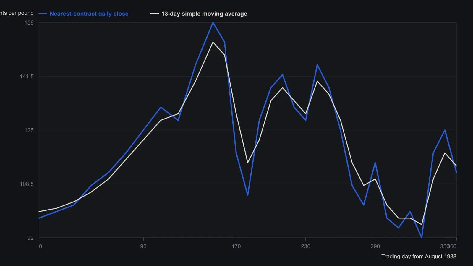
Long when the prior close is above the 13-day simple average of nearest-contract closes, otherwise cash; expiration-month contracts roll to the next nearest. Rollover days treated as cash at the prior close. Transaction costs ignored. Results are approximate.
All readings on this track · 37 readings
- 1988Constructing a lead-aware correlation coefficient
- 1989A precious-metal price as a changing intermarket equation
- 1990Two clocks for copper: a factor regime, a regression baseline, and leftover moving-average timing
- 1990Earnings yield, rate correlation and regression for equity value
- 1991Name the window, then combine leaders
- 1991Constructing a two-market linear correlation check
- 1991Constructing a commodity-bond correlation regime filter
- 1992Building intermarket context with linear correlation
- 1993Inverse-scale overlays as a gold-equity regime filter
- 1994Constructing seasonal slots from windows, analog years, and implied volatility
- 1995Pin one reference close and roll companion correlations as an overlay
- 1995Rolling correlation windows for shifting intermarket regimes
- 1998Gold as a cross-market regime barometer
- 1999The gold-bond inverse is a regime, not a cause
- 1999A nested lag test of gold leading bond yields
- 1999Constructing spreads from stock and intermarket correlation
- 2000Evaluating headline versus food-and-energy-excluded CPI as bond-yield context
- 2005A late EUR/USD fifth wave tested by the Bund-Treasury gap
- 2006Intermarket dislocation as context for short-horizon momentum
- 2008Map ordinary 12-month outcomes before stacking valuation, rates, and seasonality
- 2008A clean-energy theme inside the oil-and-energy regime
- 2014Quantitative-easing overlays as fragile belief regimes
- 2015Three intermarket checks from the late-2014 crude decline
- 2015Basket construction via rank, correlation, and locked rules
- 2015Construct a CAD-oil pair from percent-of-range Bollinger maps
- 2015CAD/USD and crude: first the correlation, then the band gap
- 2017Correlation regime versus moving-average crossover for S&P 500 exposure
- 2017Updating intermarket systems after correlation shifts
- 2017Constructing a correlation-divergence regime filter for yen and Nikkei context
- 2018Clustered negative troughs in an energy-index pairwise correlation
- 2018Filter pairwise-correlation before reading an intermarket regime
- 2018Moving-average supports in the March 2018 correlation shock
- 2020Bond spreads as an equity regime lens
- 2020Crash-protection folklore as a correlation regime question
- 2020Constructing a bounded correlation-trend-filter
- 2020Constructing a correlation-to-line trend filter
- 2020Bitcoin correlation regimes across equities and gold