2020issue C026-9
Constructing a cycle-plus-trend oscillator from a one-wavelength chord
This archive article reconstructs a cycle-plus-trend oscillator. The local trend is a straight line across one assumed wavelength, signed distances to that line become the residual sum, and a later mean-square step puts the plot in standard-deviation units.
- The construction treats the series as a cycle sitting on a trend and draws that trend as the straight line from the current close to the close one assumed cycle period earlier.
- The residual sum of signed distances to that reference line is largest at a cycle peak and most negative at a valley, so the output is described as in phase with the cycle component.
- Endpoints are left out of the average, so closes first pass through a half-period two-pole smoother. The residual average is then divided by the square root of an exponentially updated mean square.
- A horizontal line at the current close keeps the trend inside a still zero-centered oscillator, and the only length in the workflow is the assumed cycle bar count.
A cycle sitting on a straight-line trend
The construction treats the series as a cycle sitting on a trend and represents that trend as the straight line from the current close to the close one assumed cycle period earlier. That premise is a cycle-plus-trend model: the observed series is a repeating cycle sitting on a slower drift that can be drawn as a straight line across one assumed wavelength.
The assumed repeating bar-count wavelength is the dominant-cycle setting. It sets the chord length, the residual window, and the pre-smoother horizon. A 20-bar cycle length is offered as the starting lookback because the residual calculation is described as not especially sensitive to the exact wavelength, particularly near peaks and valleys.
Signed distances that stay in phase
Signed distances from each bar to the matching point on that reference line are summed over the assumed cycle length. The residual sum is the average signed distance from each bar in the lookback to the matching point on the reference line, later used as the raw oscillator. The sum is largest at a cycle peak and smallest, or most negative, at a cycle valley, so the output is described as in phase with the cycle component.
The trend-filter is a one-wavelength reference line used either as a sloped chord that subtracts the local trend or as a flat line that leaves the trend inside an oscillator.
A half-period smoother for the endpoints
The two endpoints of the reference line are left out of the average, so closes are first passed through a gentle two-pole recursive smoother whose length is set to half the assumed cycle period. That pre-filter is exponential-smoothing: recursive averaging used to gently pre-filter closes. The pre-smoother builds its coefficients from an exponential factor of 1.414 times pi over half the assumed period, then combines a two-bar average of closes with two lagged filter outputs.
Residuals in standard-deviation units
The residual average is divided by the square root of a mean-square term updated as 0.04 times the new squared sum plus 0.96 times the prior mean square, so the displayed series is scaled in standard-deviation units. That standard-deviation scale uses the same exponential-smoothing idea to maintain a mean-square scale so residuals can be expressed in volatility units rather than price units.
A flat line that keeps the trend
The trend-retaining variant replaces the sloped chord with a horizontal line at the current close, sums raw differences from that level over the same length, and still plots the result as a zero-centered oscillator. The only length used in the calculation is the bar count of the assumed cycle, so the same construction can be applied to any sampling, including intraday, tick, and volume-equivalent bars.
Reflex(20) on daily SPY through 2019
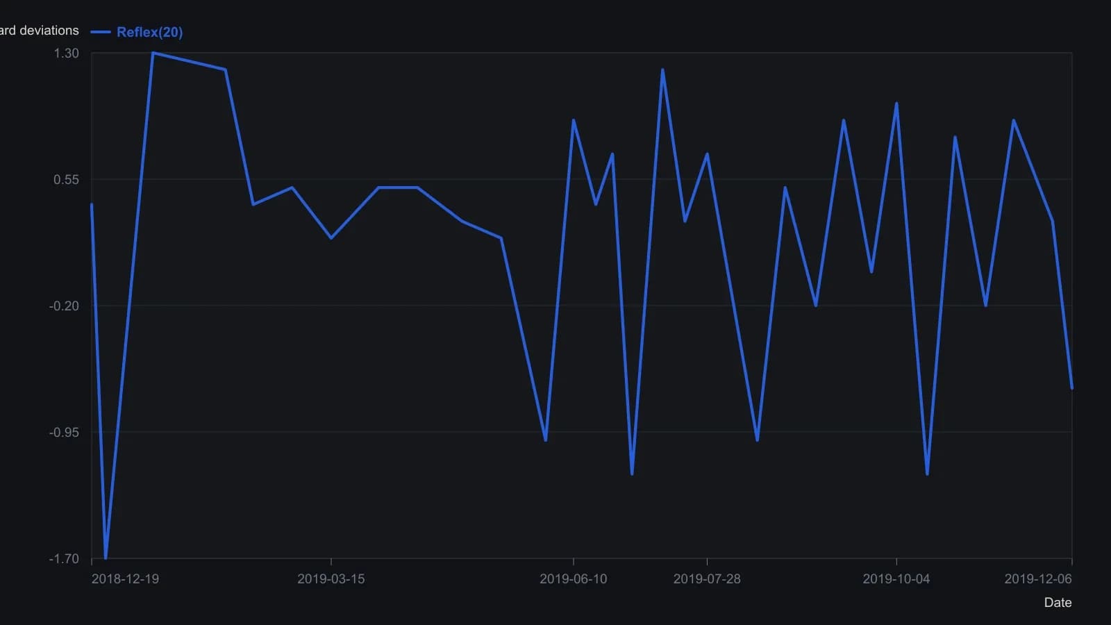
Assumed cycle length is 20 bars; a SuperSmoother of half that length is applied before the chord is fit. Vertical units are the mean residual divided by the square root of an EMA of its square (0.04 new, 0.96 prior). Digitized from the raster, so turning points are approximate to about 0.1 except the final labeled print.
All readings on this track · 31 readings
- 1982Cycle phase windows for chart signal filters
- 1987Constructing a cycle-scaled trend oscillator
- 1987Constructing a dominant-cycle grid from marked lows
- 1988Cycle lead from staggered exponential averages
- 1988Auditing the forty-month stock-price cycle
- 1989When long-wave dominant cycles cannot be disproved
- 1991Half-cycle average plot shift versus cycle attenuation
- 1991Half-cycle average contact as an amplitude-ratio test
- 1993Building a restoring-pull indicator from cycle frequency and volume
- 1995Regime filters for a dominant long wave
- 1995A cycle-tuned lead filter from bounded oscillators
- 1998Testable cycle rules instead of fear and greed
- 1999Nested Euro cycle timing as one checkable procedure
- 2002Constructing an instantaneous trendline from a dominant cycle
- 2002Half-cycle center of gravity oscillator from moving-average balance
- 2004Testing a locked forty-week cycle with a hold-or-sit-out rule
- 2005Nested timing bands for dominant-cycle confirmation
- 2005Dominant-cycle baselines versus policy-news narratives
- 2006Pairing a dominant-cycle horizon with trend and oscillators
- 2006A dominant-cycle split into a trend filter and residual Relative Strength Index
- 2007Construct a momentum difference from the dominant cycle
- 2007Naive dominant-cycle rules fail without crowd tests
- 2012Constructing a dominant-cycle forecast as a timing window
- 2012Open-parameter construction of dominant-cycle baselines
- 2013Using a second-term election to check a predeclared dominant-cycle forecast
- 2014Constructing a dominant-cycle forecast baseline
- 2014Quotient transform as an early-onset trend filter
- 2014Construct a trough-to-trough cycle map with the Detrended Price Oscillator
- 2015Dominant-cycle alignment before an earnings catalyst
- 2017Causal reverse exponential average for cycle and trend
- 2020Constructing a cycle-plus-trend oscillator from a one-wavelength chord