1993issue C101-2
Building a restoring-pull indicator from cycle frequency and volume
A restoring-pull indicator converts each session’s cycle length into angular frequency, weights that frequency by the session’s volume, and then steadies the raw series with an exponential average calibrated to a simple moving average.
- Cycle length is a market-specific input that can change from day to day, so it must be estimated for each session before a restoring-pull value is formed.
- Angular frequency is two times pi divided by the current cycle length, and frequency is treated as the reciprocal of that length.
- The raw restoring-pull value multiplies session volume by the square of that session’s angular frequency.
- A six-period exponential average with smoothing constant 0.2857 is applied so the smoother matches a six-day simple moving average.
What the indicator constructs
A restoring-pull indicator is a constructed series that combines a market’s current cycle length with that session’s volume, then typically smooths the result.
Cycle length is treated as a market-specific input that can change from day to day. It must be estimated for each session before a restoring-pull value can be formed.
Convert cycle length into angular frequency
Angular frequency is formed by dividing two times pi by the current cycle length. Frequency itself is treated as the reciprocal of that length.
Because the length can change from session to session, the frequency used in the construction is taken from the latest estimated cycle length rather than held fixed.
Weight frequency by session volume
The restoring-pull construction multiplies session volume by the square of angular frequency taken from that session’s cycle length. The product is one raw restoring-pull observation for the session.
Stabilize the raw series with exponential smoothing
The unsmoothed daily restoring-pull series is described as erratic, so a six-period exponentially smoothed moving average is applied to it.
Exponential smoothing is a recursive average that blends today’s raw restoring-pull value with yesterday’s smoothed value using a fixed smoothing constant. The smoothing constant 0.2857 is specified so the smoother matches a six-day simple moving average.
How the exponential average can be started
The exponential average may be started by copying the first raw observation, or by first computing a simple moving average and then switching to the recursive update.
The second path is a simple-moving-average seed. A short simple average of the raw series is built first, then the recursion takes over.
A historical pairing of volume and cycle length
A worked example builds the series from paired daily volume and cycle-length observations on the June 1993 Standard & Poor’s futures contract.
June 1993 S&P futures — raw RPI versus six-day EMA
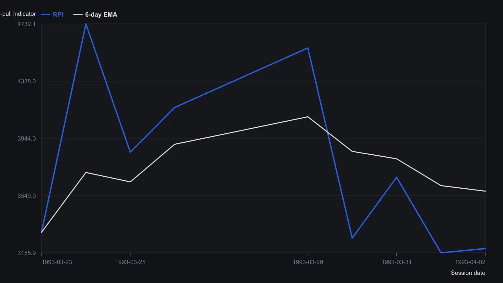
The exponential average uses smoothing constant 0.2857, chosen to match a six-session simple moving average, and is seeded by copying the first session’s raw RPI.
All readings on this track · 31 readings
- 1982Cycle phase windows for chart signal filters
- 1987Constructing a cycle-scaled trend oscillator
- 1987Constructing a dominant-cycle grid from marked lows
- 1988Cycle lead from staggered exponential averages
- 1988Auditing the forty-month stock-price cycle
- 1989When long-wave dominant cycles cannot be disproved
- 1991Half-cycle average plot shift versus cycle attenuation
- 1991Half-cycle average contact as an amplitude-ratio test
- 1993Building a restoring-pull indicator from cycle frequency and volume
- 1995Regime filters for a dominant long wave
- 1995A cycle-tuned lead filter from bounded oscillators
- 1998Testable cycle rules instead of fear and greed
- 1999Nested Euro cycle timing as one checkable procedure
- 2002Constructing an instantaneous trendline from a dominant cycle
- 2002Half-cycle center of gravity oscillator from moving-average balance
- 2004Testing a locked forty-week cycle with a hold-or-sit-out rule
- 2005Nested timing bands for dominant-cycle confirmation
- 2005Dominant-cycle baselines versus policy-news narratives
- 2006Pairing a dominant-cycle horizon with trend and oscillators
- 2006A dominant-cycle split into a trend filter and residual Relative Strength Index
- 2007Construct a momentum difference from the dominant cycle
- 2007Naive dominant-cycle rules fail without crowd tests
- 2012Constructing a dominant-cycle forecast as a timing window
- 2012Open-parameter construction of dominant-cycle baselines
- 2013Using a second-term election to check a predeclared dominant-cycle forecast
- 2014Constructing a dominant-cycle forecast baseline
- 2014Quotient transform as an early-onset trend filter
- 2014Construct a trough-to-trough cycle map with the Detrended Price Oscillator
- 2015Dominant-cycle alignment before an earnings catalyst
- 2017Causal reverse exponential average for cycle and trend
- 2020Constructing a cycle-plus-trend oscillator from a one-wavelength chord