1995issue C061-7
A cycle-tuned lead filter from bounded oscillators
A bounded oscillator is locked to the dominant cycle, centered, and differenced against a short exponential average to form a residual that leads the oscillator. The construction is used only while amplitude stays limited and median crossings stay regular.
- Lock a bounded oscillator to the dominant cycle until the series is sine-like and median crossings stay regular.
- Center the oscillator, then subtract a short exponential average whose induced lag is one-eighth of that cycle.
- Read crossings of the residual against the oscillator, and add extra smoothing only if those crossings are too noisy.
- Set the residual aside when a stochastic stays pinned near an extreme or the Poisson-like crossing count cannot be met.
The residual as a construction
The optimum predictive filter is the residual formed by subtracting an exponential moving average from a centered, amplitude-limited oscillator and reading crossings against that oscillator. In the historical workflow the filter is constructed as the difference between an amplitude-limited indicator and that indicator's exponential moving average.
After the oscillator is centered, the residual is overlaid on it. Crossings of residual versus oscillator are the stated signal rule. Extra smoothing may be applied first if those crossings are too noisy.
Validity, detrending, and the dominant cycle
The construction is treated as valid only when the source indicator has limited amplitude swings and its median crossings, after proper detrending, are consistent with a Poisson-like count of zero crossings. That Poisson zero-crossing requirement is approximated only after prices are properly detrended.
Detrending means shortening or lengthening the oscillator observation window until swings just reach the 0 and 1 bounds and median crossings stay regular. The dominant cycle is the interval between successive peaks or troughs used to set oscillator lookback and exponential-average lag so the waveform is detrended and roughly sinusoidal.
Two bounded oscillators
Relative strength index, written as closes-up over the sum of closes-up and closes-down, is bounded between 0 and 1 and is recentered on zero by subtracting 0.5. From a cyclical view, relative strength index is treated as properly detrended when the observation period lies between a half cycle and a full cycle.
The stochastic oscillator is likewise bounded between 0 and 1, equaling 1 when the close is at the lookback high and 0 when the close is at the lookback low. A stochastic is more often properly detrended near one full cycle. When a stochastic remains pinned near an extreme, the series is described as trend mode, the probability constraint cannot be met, and the predictive construction is to be set aside rather than forced.
Lag as a fraction of the cycle
A tabulated construction rule sets induced exponential-average lag at one-eighth of a cycle (45 degrees), at which the average and the residual each have amplitude about 0.7 times the oscillator. An exponential-average constant of 0.25, a three-day induced lag, is offered as a default expected to be reasonable for cycle lengths from 12 to 24 days.
An exponential moving average is a recursive smoother whose constant sets induced lag. Very short lag increases theoretical lead but shrinks residual amplitude.
EMA lag versus predictor lead as delay grows
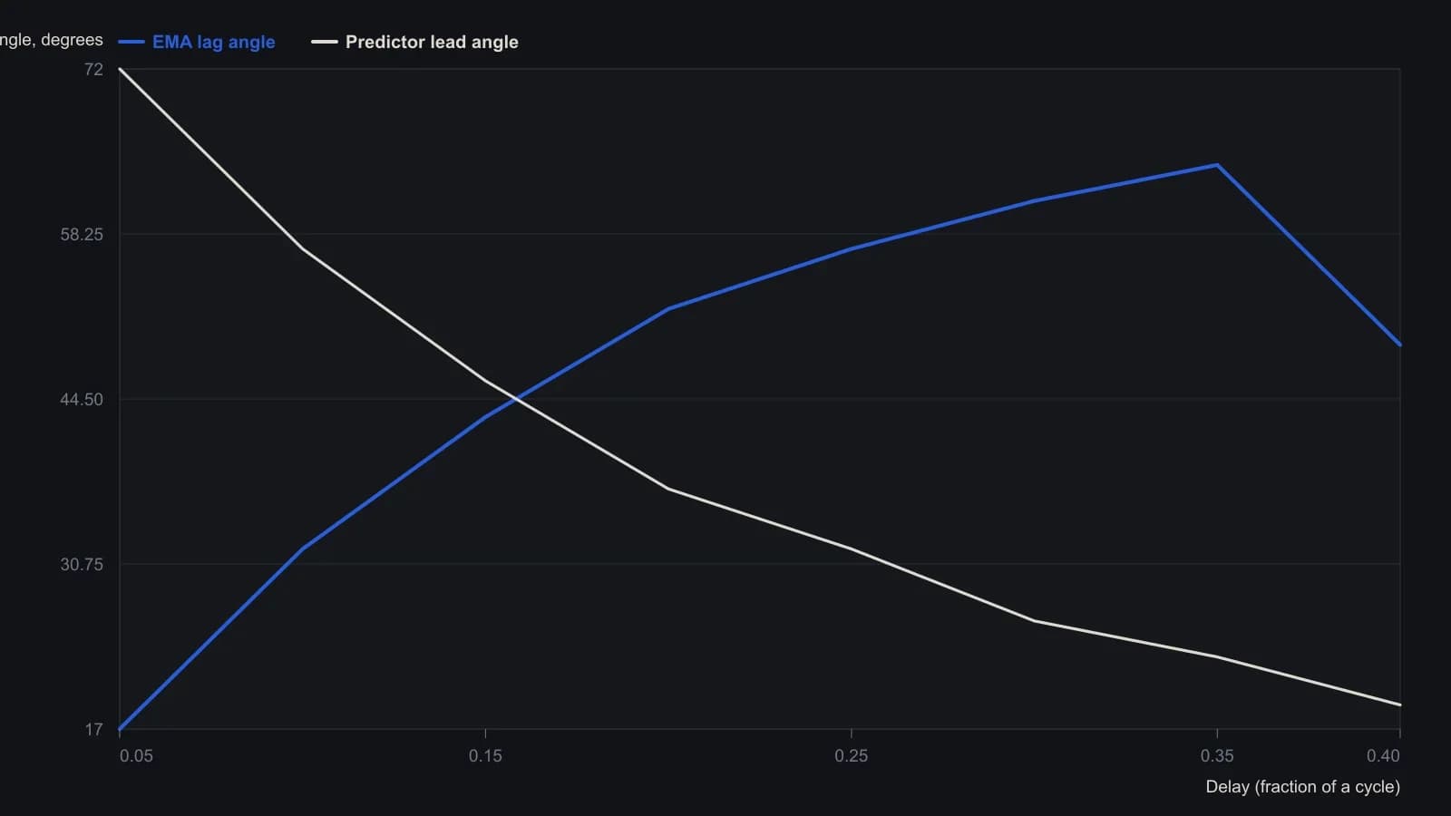
Delay is the intended EMA lag as a fraction of one full cycle. The source notes EMA lag never reaches a quarter cycle (90°) and that a very short lag gives near-maximum lead but a tiny predictor amplitude.
A controlled sine-series check
On a 24-bar sine test series, a 12-bar relative-strength lookback (half cycle) and a 0.25 exponential-average constant (one-eighth-cycle induced lag) produced a smaller-amplitude residual that led the oscillator. Typical lead is described as about one-eighth of a cycle, which is a one-day advance on an eight-day cycle and may arrive early enough on longer cycles that an entry is delayed by a day or two.
All readings on this track · 31 readings
- 1982Cycle phase windows for chart signal filters
- 1987Constructing a cycle-scaled trend oscillator
- 1987Constructing a dominant-cycle grid from marked lows
- 1988Cycle lead from staggered exponential averages
- 1988Auditing the forty-month stock-price cycle
- 1989When long-wave dominant cycles cannot be disproved
- 1991Half-cycle average plot shift versus cycle attenuation
- 1991Half-cycle average contact as an amplitude-ratio test
- 1993Building a restoring-pull indicator from cycle frequency and volume
- 1995Regime filters for a dominant long wave
- 1995A cycle-tuned lead filter from bounded oscillators
- 1998Testable cycle rules instead of fear and greed
- 1999Nested Euro cycle timing as one checkable procedure
- 2002Constructing an instantaneous trendline from a dominant cycle
- 2002Half-cycle center of gravity oscillator from moving-average balance
- 2004Testing a locked forty-week cycle with a hold-or-sit-out rule
- 2005Nested timing bands for dominant-cycle confirmation
- 2005Dominant-cycle baselines versus policy-news narratives
- 2006Pairing a dominant-cycle horizon with trend and oscillators
- 2006A dominant-cycle split into a trend filter and residual Relative Strength Index
- 2007Construct a momentum difference from the dominant cycle
- 2007Naive dominant-cycle rules fail without crowd tests
- 2012Constructing a dominant-cycle forecast as a timing window
- 2012Open-parameter construction of dominant-cycle baselines
- 2013Using a second-term election to check a predeclared dominant-cycle forecast
- 2014Constructing a dominant-cycle forecast baseline
- 2014Quotient transform as an early-onset trend filter
- 2014Construct a trough-to-trough cycle map with the Detrended Price Oscillator
- 2015Dominant-cycle alignment before an earnings catalyst
- 2017Causal reverse exponential average for cycle and trend
- 2020Constructing a cycle-plus-trend oscillator from a one-wavelength chord