2012issue C0442-48
Constructing a dominant-cycle forecast as a timing window
A dominant-cycle model is assembled from the longest rhythm downward, tracked with multi-lookback price-velocity, and published as a statistical turn-window on the time axis rather than as a price target.
- Start with the longest rhythm on the longest available ordered series, then layer two or three named embedded cycles beneath that dominant cycle.
- Construction has three layers: a number-based cycle length, statistical checks of central tendency and standard deviation, and tracking tools that flag turns as they form.
- Plot price-velocity over at least three lookbacks to track the cycle, and build trend separately as current price expressed as a percentage of range.
- Issue a turn-window scored with one-, two-, and three-standard-deviation bands. The forecast times a possible trend change and does not state move size.
This article reconstructs how a dominant-cycle forecast is put together. The finished product is a turn-window: a statistically bounded interval on the time axis where a cycle is due to change. It does not specify the size of the subsequent move.
Isolate the longest rhythm first
A dominant-cycle model is built top-down. The longest rhythm on the longest available ordered series is identified first. Shorter embedded cycles are then layered beneath it. Embedded cycles are typically modeled as two or three named subcomponents inside the dominant cycle.
Cycle identification starts with visual inspection of an ordered series, then statistical analysis and regression modeling. The genesis-point is the first observation from which a given cycle is treated as existing.
The constructed cycle is not required to keep a constant period. It may skip iterations, stretch, compress, or recombine into a new cycle.
Build in three layers
Construction uses three layers. The first is a number-based derivation of cycle length. The second is statistical checks of central tendency and standard deviation. The third is tracking tools that flag turns as they form.
Instrument the cycle with price-velocity
Cycle tracking uses price-velocity over at least three lookbacks plotted together. Price-velocity is current price versus price a fixed number of periods earlier. That tracker measures the cycle under study, not the trend.
Trend is constructed separately, preferably as the current price expressed as a percentage of the range over a chosen lookback.
Read translation, then publish a turn-window
In advances the cycle crest is expected to the right of midpoint. In declines it is expected to the left. That shift is translation.
The cycle forecast is a window on the time axis for a possible trend change. Historical turns are scored against the projected date with one-, two-, and three-standard-deviation bands, corresponding to about 68 percent, 95 percent, and 99 percent of observations.
S&P 500 cash percentage-range, Dec 2010–Mar 2012
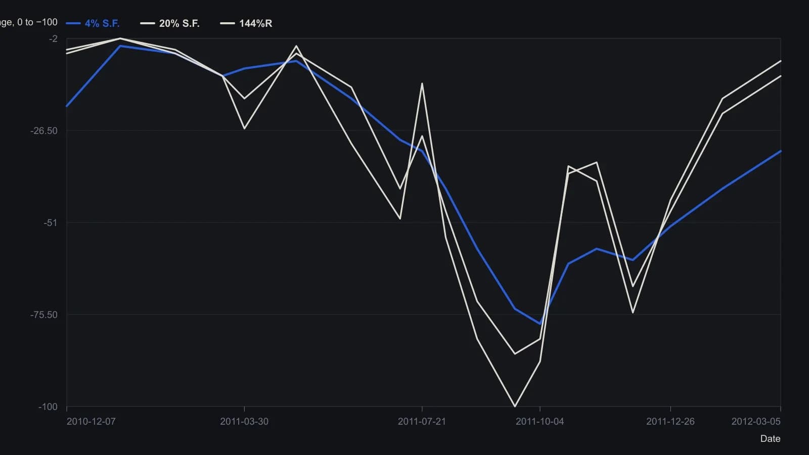
Y follows the source figure’s 0 (top of the lookback range) to −100 (bottom of the range) scale. Series names match the printed legend. Values are digitised from a magazine raster, so turning-point levels are only good to a few percentage-range points.
All readings on this track · 31 readings
- 1982Cycle phase windows for chart signal filters
- 1987Constructing a cycle-scaled trend oscillator
- 1987Constructing a dominant-cycle grid from marked lows
- 1988Cycle lead from staggered exponential averages
- 1988Auditing the forty-month stock-price cycle
- 1989When long-wave dominant cycles cannot be disproved
- 1991Half-cycle average plot shift versus cycle attenuation
- 1991Half-cycle average contact as an amplitude-ratio test
- 1993Building a restoring-pull indicator from cycle frequency and volume
- 1995Regime filters for a dominant long wave
- 1995A cycle-tuned lead filter from bounded oscillators
- 1998Testable cycle rules instead of fear and greed
- 1999Nested Euro cycle timing as one checkable procedure
- 2002Constructing an instantaneous trendline from a dominant cycle
- 2002Half-cycle center of gravity oscillator from moving-average balance
- 2004Testing a locked forty-week cycle with a hold-or-sit-out rule
- 2005Nested timing bands for dominant-cycle confirmation
- 2005Dominant-cycle baselines versus policy-news narratives
- 2006Pairing a dominant-cycle horizon with trend and oscillators
- 2006A dominant-cycle split into a trend filter and residual Relative Strength Index
- 2007Construct a momentum difference from the dominant cycle
- 2007Naive dominant-cycle rules fail without crowd tests
- 2012Constructing a dominant-cycle forecast as a timing window
- 2012Open-parameter construction of dominant-cycle baselines
- 2013Using a second-term election to check a predeclared dominant-cycle forecast
- 2014Constructing a dominant-cycle forecast baseline
- 2014Quotient transform as an early-onset trend filter
- 2014Construct a trough-to-trough cycle map with the Detrended Price Oscillator
- 2015Dominant-cycle alignment before an earnings catalyst
- 2017Causal reverse exponential average for cycle and trend
- 2020Constructing a cycle-plus-trend oscillator from a one-wavelength chord