2014issue C0826-29
Quotient transform as an early-onset trend filter
The archive workflow band-limits an oscillator with a roofing filter, peak-normalizes it, remaps it with a quotient transform, and then applies either a paired zero-cross rule or a dominant-cycle slope comparison.
- Any oscillator is translated and dilated into the interval from -1 to +1 before the quotient transform, after a roofing filter has already removed long wavelengths plus aliasing and the highest remaining frequencies.
- The k-parameter sets how strongly the mapped output stays positive or negative across the input range, so the filter's time on one side of zero is an explicit choice rather than a byproduct of spectral dilation.
- After automatic gain control, the unmapped roofing filter is assigned a short-term swing role because of residual wiggles, while the same series after the quotient map is assigned the trend-onset role.
- A higher-K early-onset zero-cross can be paired with a milder-K exit, or trend slope over one dominant-cycle period can be compared with that cycle's peak-to-peak amplitude, so onset and hold duration are not the same object.
The historical workflow
The archive describes a historical workflow for a trend filter. A roofing filter first band-limits the input. Automatic gain control then peak-normalizes the filtered series. A quotient transform remaps that bounded series so its sign relative to zero is treated as the trend state.
The quotient transform is the rational map of a bounded input plus K, divided by K times that input plus 1, with K strictly inside the open interval from -1 to 1. It nonlinearly biases an oscillator that has already been placed in the interval from -1 to +1.
Bound and band-limit the oscillator
Spectral dilation is the tendency of swing amplitude to grow with cycle period, so shorter sampling intervals show smaller swings than longer ones. The roofing filter addresses that tendency before any later mapping. It is a two-stage band-limit: a two-pole high-pass removes long wavelengths, and a SuperSmoother removes aliasing and the highest remaining frequencies.
The worked construction retains cyclic components shorter than 100 bars and SuperSmoothes with a default low-pass period of 30. It then applies automatic gain control. That peak tracker scales the latest filtered value by a slowly decaying record of recent absolute extrema rather than a fixed lookback range. The automatic-gain peak decays by 0.991 each bar.
Any oscillator fed to the later map must first be translated and dilated into the interval from -1 to +1. One stated CCI route is division by 200 with clipping. One stated stochastic or RSI route is subtract 50 then divide by 50.
Set one K for time on one side of zero
After peak normalization, the unmapped roofing filter is assigned a short-term swing role because of residual wiggles. The same series after the quotient map is assigned the trend-onset role.
The k-parameter is the open-interval constant that sets how strongly the quotient map stays positive or negative across the input range. With K set to 0.8, a zero input maps to 0.8, the output stays positive until the input reaches -0.8, and more negative inputs then drive the output rapidly toward -1. The worked construction applies the quotient map with a default K of 0.85.
Positive K values keep the mapped output positive over most of the input range and are used when the construction assumes an upside bias. Negative K values reverse that symmetry for a downside bias. The same k-parameter can be set separately for onset and exit.
Keep onset and hold as separate rules
A rule-based entry is a paired zero-cross procedure that opens a long when a higher-K quotient series crosses above zero and exits when a lower-K series crosses below zero. In the stated long procedure, the higher-K early-onset series is the entry object, and the position is held until a second series with K set to 0.4 crosses below zero.
An alternative classifier measures trend slope over one dominant-cycle period against that cycle's peak-to-peak amplitude. The dominant cycle is the measured cycle period used as that lookback. The comparison labels the state as uptrend, downtrend, or sideways.
Quotient transform transfer response for selected K
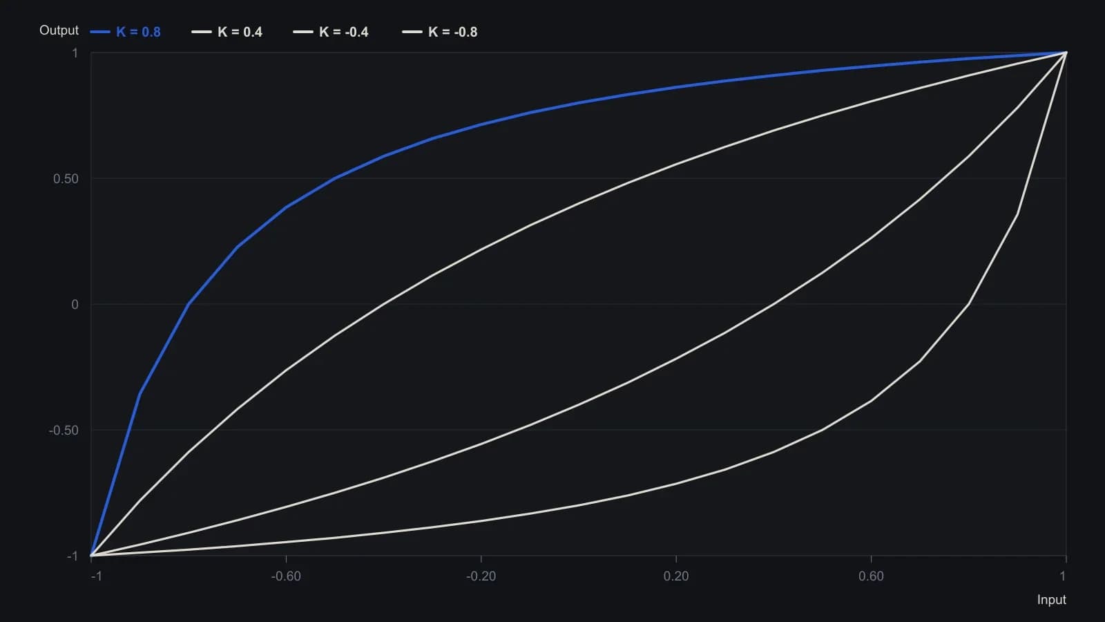
The source plots six K values; only four are shown here to stay within the series limit. Endpoints at Input = ±1 map to Output = ±1 for every K.
All readings on this track · 31 readings
- 1982Cycle phase windows for chart signal filters
- 1987Constructing a cycle-scaled trend oscillator
- 1987Constructing a dominant-cycle grid from marked lows
- 1988Cycle lead from staggered exponential averages
- 1988Auditing the forty-month stock-price cycle
- 1989When long-wave dominant cycles cannot be disproved
- 1991Half-cycle average plot shift versus cycle attenuation
- 1991Half-cycle average contact as an amplitude-ratio test
- 1993Building a restoring-pull indicator from cycle frequency and volume
- 1995Regime filters for a dominant long wave
- 1995A cycle-tuned lead filter from bounded oscillators
- 1998Testable cycle rules instead of fear and greed
- 1999Nested Euro cycle timing as one checkable procedure
- 2002Constructing an instantaneous trendline from a dominant cycle
- 2002Half-cycle center of gravity oscillator from moving-average balance
- 2004Testing a locked forty-week cycle with a hold-or-sit-out rule
- 2005Nested timing bands for dominant-cycle confirmation
- 2005Dominant-cycle baselines versus policy-news narratives
- 2006Pairing a dominant-cycle horizon with trend and oscillators
- 2006A dominant-cycle split into a trend filter and residual Relative Strength Index
- 2007Construct a momentum difference from the dominant cycle
- 2007Naive dominant-cycle rules fail without crowd tests
- 2012Constructing a dominant-cycle forecast as a timing window
- 2012Open-parameter construction of dominant-cycle baselines
- 2013Using a second-term election to check a predeclared dominant-cycle forecast
- 2014Constructing a dominant-cycle forecast baseline
- 2014Quotient transform as an early-onset trend filter
- 2014Construct a trough-to-trough cycle map with the Detrended Price Oscillator
- 2015Dominant-cycle alignment before an earnings catalyst
- 2017Causal reverse exponential average for cycle and trend
- 2020Constructing a cycle-plus-trend oscillator from a one-wavelength chord