1988issue C101-4
Auditing the forty-month stock-price cycle
A 40.68-month stock-price cycle specified by 1951 can be locked as a template. Later turning points are then scored only after trend removal, and a weighted-average rerun is treated as a length check rather than a live price call.
- Lock the 40.68-month length and phase first, then use later data only to test post-discovery-continuation of that same dominant-cycle.
- Score later turning points after a trend-filter. A raw-price overlay can make a scheduled decline look sideways until prices are expressed as departures around trend.
- Treat a weighted-moving-average rerun as a length and timing check. It can corroborate the 1951 period, but it drops months at both ends of the sample and is not a live price call.
- An ideal-schedule is a timing ruler. The 40.68-month rhythm was only one concurrent cycle, so any forecast would have required the other components and the surrounding trend.
Lock the published template
Editorial: this article teaches a post-discovery cycle audit. The published 40.68-month template is locked, later turning points are scored only after trend removal, and a weighted-average rerun is treated as a length check rather than a live price call.
A 40.68-month stock-price cycle had been specified by 1951, and later updates were used to judge whether the same rhythm still followed the extended average pattern after that definition. Editorial: that is a test of post-discovery-continuation. The length and phase stay fixed, and later data are scored against that template instead of being used to rewrite it.
A crest-to-crest interval of about 40 to 41 months in market averages had long been noted, and at times the rhythm was strong enough to be seen by inspection before trend removal or other filtering. Once that length and phase were fixed, the series was treated as a dominant-cycle, the leading periodic component under review.
Use the ideal-schedule as a ruler
Several repetitions in the 1950s and 1960s lined up poorly with the ideal 40.68-month schedule, while the most recent five up or down legs were described as visible even in the unadjusted series.
The ideal schedule placed a turning point in July 1987, and monthly average prices were reported to have crested the following August. The next ideal turning point on that schedule was a low at March 1989, presented as a timing benchmark for the cycle rather than a forecast of the market.
Score later turns only after a trend-filter
A raw-price overlay was called an inaccurate evaluation method because the cycle was defined on detrended and filtered data. The span from the February 1984 ideal crest to the November 1985 ideal trough looked more sideways than downward until those observations were expressed as departures around trend.
Editorial: later turning points are scored only after a trend-filter. The cycle is then read as departures around a local trend instead of in raw prices.
Treat a weighted average as a length check
Later work with weighted moving averages was said to corroborate the 1951 length and timing, at the cost of losing many months of data at each end of the series.
Editorial: a weighted-moving-average rerun can reconfirm a previously measured period. It is a length check, not a live price call, and it discards observations at both ends of the sample.
Read filtered-move lengths, not raw legs
In the detrended and filtered history compiled since 1789, a 20-month up or down move was the most common length. Those spans are filtered-move readings, measured in the isolated cycle series rather than in unadjusted market prices. 35 of 117 moves lasted exactly 20 months, 79 percent lasted 16 to 22 months, and observed lengths ranged from 9 to 29 months.
Average amplitude of the isolated cycle over that history was given as about 12 percent to 13 percent of trend, with a note that a sharp 1987 spike could pull that average away from a more typical reading.
Filtered 40.68-month cycle: length of up and down moves, 1789 onward
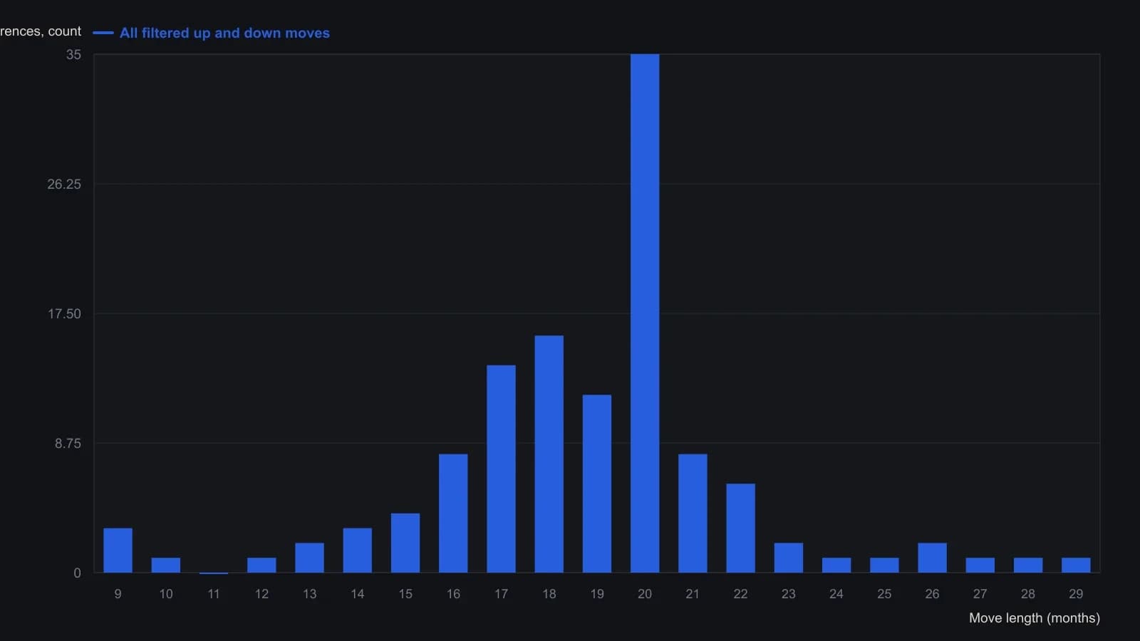
Lengths are measured in the detrended, filtered cycle series, not in actual stock prices. The source gives the 20-month bar exactly (35 of 117); neighbouring bars are approximate readings from the printed histogram. Average cycle amplitude is stated separately as about 12–13% of trend and is not plotted here.
Keep concurrent cycles in view
The 40.68-month rhythm was treated as only one of several concurrent cycles, and the 1987 decline was also linked to a 50-year cycle, so any forecast would have required combining those components with a view of the surrounding trend.
All readings on this track · 31 readings
- 1982Cycle phase windows for chart signal filters
- 1987Constructing a cycle-scaled trend oscillator
- 1987Constructing a dominant-cycle grid from marked lows
- 1988Cycle lead from staggered exponential averages
- 1988Auditing the forty-month stock-price cycle
- 1989When long-wave dominant cycles cannot be disproved
- 1991Half-cycle average plot shift versus cycle attenuation
- 1991Half-cycle average contact as an amplitude-ratio test
- 1993Building a restoring-pull indicator from cycle frequency and volume
- 1995Regime filters for a dominant long wave
- 1995A cycle-tuned lead filter from bounded oscillators
- 1998Testable cycle rules instead of fear and greed
- 1999Nested Euro cycle timing as one checkable procedure
- 2002Constructing an instantaneous trendline from a dominant cycle
- 2002Half-cycle center of gravity oscillator from moving-average balance
- 2004Testing a locked forty-week cycle with a hold-or-sit-out rule
- 2005Nested timing bands for dominant-cycle confirmation
- 2005Dominant-cycle baselines versus policy-news narratives
- 2006Pairing a dominant-cycle horizon with trend and oscillators
- 2006A dominant-cycle split into a trend filter and residual Relative Strength Index
- 2007Construct a momentum difference from the dominant cycle
- 2007Naive dominant-cycle rules fail without crowd tests
- 2012Constructing a dominant-cycle forecast as a timing window
- 2012Open-parameter construction of dominant-cycle baselines
- 2013Using a second-term election to check a predeclared dominant-cycle forecast
- 2014Constructing a dominant-cycle forecast baseline
- 2014Quotient transform as an early-onset trend filter
- 2014Construct a trough-to-trough cycle map with the Detrended Price Oscillator
- 2015Dominant-cycle alignment before an earnings catalyst
- 2017Causal reverse exponential average for cycle and trend
- 2020Constructing a cycle-plus-trend oscillator from a one-wavelength chord