1991issue C071-7
Ranked half-year rate changes as an equity signal filter
First place the latest 26-week long Treasury yield change into a four-group rank. Then decide whether an independent equity technical reading is allowed to fire.
- Long-term rate moves and equity prices were treated as inversely linked for two reasons: lower corporate funding costs, and a shift of capital away from less attractive long-term debt.
- Each week from 1955 through 1989, the halfYearYieldChange was ranked from the largest decline to the largest rise and split into four rateChangeQuartile groups.
- Later equity-index results moved opposite the ranked rate change, larger rate moves sat with larger average subsequent equity moves, and that inverseRateEquityLink appeared in each 20-year window that was checked.
- A regimeGatedSignal acts on a separate equity technical forecast only when the current rate-change rank is above average, and otherwise abstains.
How the rate rank is used
The archive workflow ranks a rolling 26-week long-yield change first, then sets that rank beside a separate equity technical forecast. The rate side is a condition set, not a replacement price signal.
Editorial: treat the rank as a permission layer. Compute the halfYearYieldChange, assign the rateChangeQuartile, and only then ask whether the independent technical reading may fire.
Why the inverse link was used
Long-term rate moves and equity prices were treated as inversely linked for two distinct reasons. Lower long-term rates reduce corporate funding costs. They also make long-term debt less attractive, so capital can shift away from that debt.
Building the half-year yield change
Each week from 1955 through 1989, the percent change in the long Treasury yield over the prior 26 weeks was computed. That rolling reading is the halfYearYieldChange.
The yields sit on a splicedLongYieldSeries. The history joins long government yields through 1961, the 20-year constant-maturity yield through mid-1977, and the 30-year constant-maturity yield thereafter.
Ranking later equity results
Those weekly readings were ranked from the largest decline to the largest rise and split into four groups. Each group is a rateChangeQuartile.
For each ranked group, the next 26-week equity-index change was summarized as a geometric average that was annualized by doubling, and as the share of those half-year windows that finished higher. Dividends were left out.
In the full sample, later equity-index results moved opposite the ranked rate change, and larger rate moves sat with larger average subsequent equity moves. That inverseRateEquityLink appeared in each 20-year market window that was checked.
S&P 500 payoff after ranked 26-week Treasury yield changes
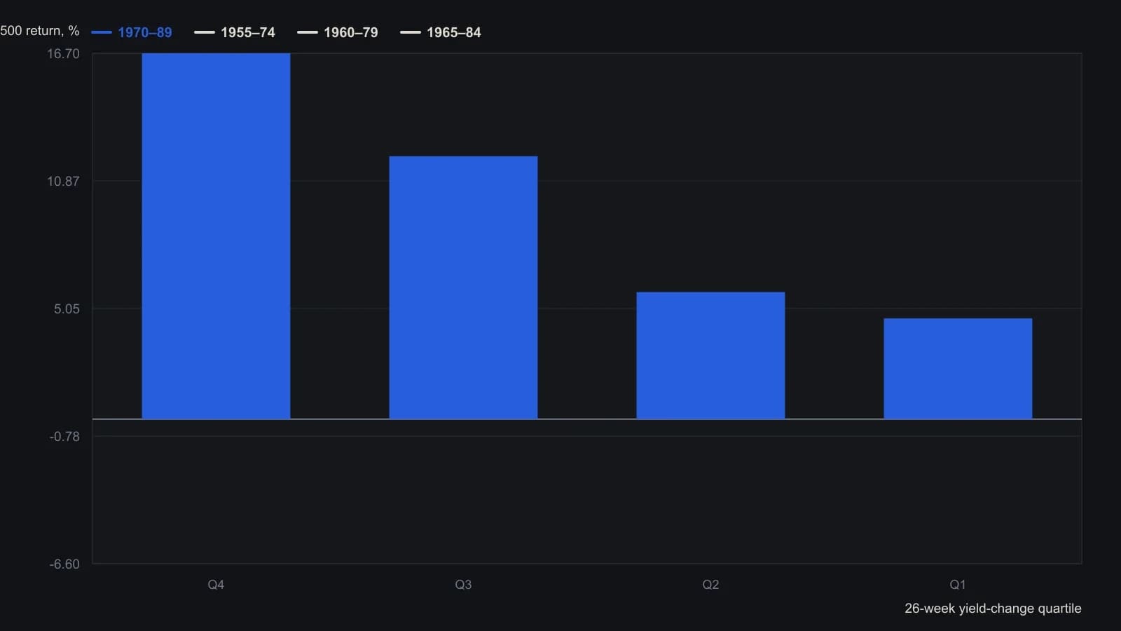
Each listed span is a 20-year window and overlaps the next. The source annualized the geometric 26-week S&P 500 mean by multiplying by two. Quartile 4 is the largest 26-week decline in the long Treasury yield; quartile 1 is the largest rise.
When the technical reading may fire
A two-way ranking grid places the current technical forecast against the rate-defined condition set. It withholds those technical actions when the rate backdrop is below or well below average.
Editorial: this grid is the regimeGatedSignal. It acts on the separate equity technical forecast only when the current rate-change rank is above average, and otherwise abstains.
All readings on this track · 41 readings
- 1989Evaluating venue volume as a speculation-breadth signal
- 1991A thirty-name price-weighted average as a seasonal regime classroom
- 1991Ranked half-year rate changes as an equity signal filter
- 1991Demographic wave as a market-regime overlay
- 1994Seasonal range regimes as a futures context overlay
- 1996Evaluating presidential party terms as equity regimes
- 1996A dominant cycle is a baseline, not a reprint
- 1996Seasonality and presidential election cycle regimes
- 1997Stacking calendar regimes around election years
- 1997Calendar seasonality as a testable trading procedure
- 1997Lunar phase delay as a testable seasonal regime
- 1998Seasonal system construction without curve-fitting
- 1999Crowd life cycle as a market regime map
- 2001Regime-dependent cycle timing after four-year and seasonal lows
- 2002A 2002 case study in regime-first seasonal selection
- 2002Seasonal windows and dominant-cycle rules
- 2002Fifty-four-year wholesale cycle as an inflation-deflation regime map
- 2004The championship conference rule as a yearly regime case study
- 2004Election-year seasonality as trade regime context
- 2006Two-ten inversion as an intermarket regime filter
- 2006Midterm-to-presidential seasonal holding window
- 2008Two-layer equity regimes from seasonality and price history
- 2008Seasonal futures as a regime filter, not a calendar rule
- 2008Retesting seasonal rules when regimes change
- 2010Corn and wheat staggered calendars as dollar-neutral seasonal spreads
- 2011Name the S&P 500 trend regime before using weekly and monthly seasonality
- 2012Seasonal windows that wait for confirmation
- 2013Pair-sleeve rotation as a two-state sector regime-switch
- 2013Lunar phase as a seasonal overlay on implied volatility
- 2013Soybean seasonal highs in a five-year carryover regime
- 2014Year-end tax-loss selling as a seasonal regime
- 2017Calendar-window overlays that mute mechanical signals without rewriting the system
- 2017A four-year cycle and volume case study of a secular bear
- 2017Treat the valuation climate as climate and implied-volatility extremes as weather
- 2019Seasonal depth versus tracking for futures position sizing
- 2019Stacking cycle forecasts with seasonal regimes
- 2019Hit-rate gates for seasonal regime evaluation
- 2019July to October as a seasonal window, not a reason to own the name
- 2020A recession-regime checklist from valuation stretch and the yield curve
- 2020Treat a seasonal idea as a stay-or-sit holding procedure
- 2020A single position as a sleeve on a seasonal regime map