2019issue C0920-23
Hit-rate gates for seasonal regime evaluation
A yearly-average seasonal map can rank a month as the seasonal high when a few standout years dominate. Positive-return frequency, a rolling four-year window, and a consistency gate turn that map into a regime overlay that can stay flat.
- A yearly-average seasonal map can rank a month as the seasonal high when a few standout years dominate, even if that month is ordinary in most other years.
- Positive-return frequency counts only whether a month was above zero, and that count is used to judge whether a seasonal peak or trough is consistent.
- A rolling four-year window and a consistency gate allow seasonal abstention when the map is too muted to show one reliably strong month and one reliably weak month.
- Because the frequency rules do not follow trend or momentum logic, they are framed as a diversification sleeve rather than a substitute for those approaches.
What a yearly-average seasonal map measures
A yearly-average seasonal map is built by scaling each month’s price to that year’s mean, subtracting one, and then averaging those scaled values across years by calendar month. The map is a calendar profile of how each month sits relative to that year’s average price.
A month can rank as the seasonal high on average returns because a few standout years dominate, even when that month is ordinary in most other years. Average size and year-to-year regularity are different questions.
Positive-return frequency
Counting how often a month’s return is merely positive, regardless of size, is used to judge whether a seasonal peak or trough is consistent. That share is the positive-return frequency.
In the corn frequency illustration, February, March, and April each show an 80 percent chance of a positive monthly return, versus 10 percent in October. The airline-equity frequency illustration, using 13 years beginning in 2006, stays inside a 40-to-60 percent band and therefore shows less calendar conviction than the futures example.
Corn monthly positive-return frequency
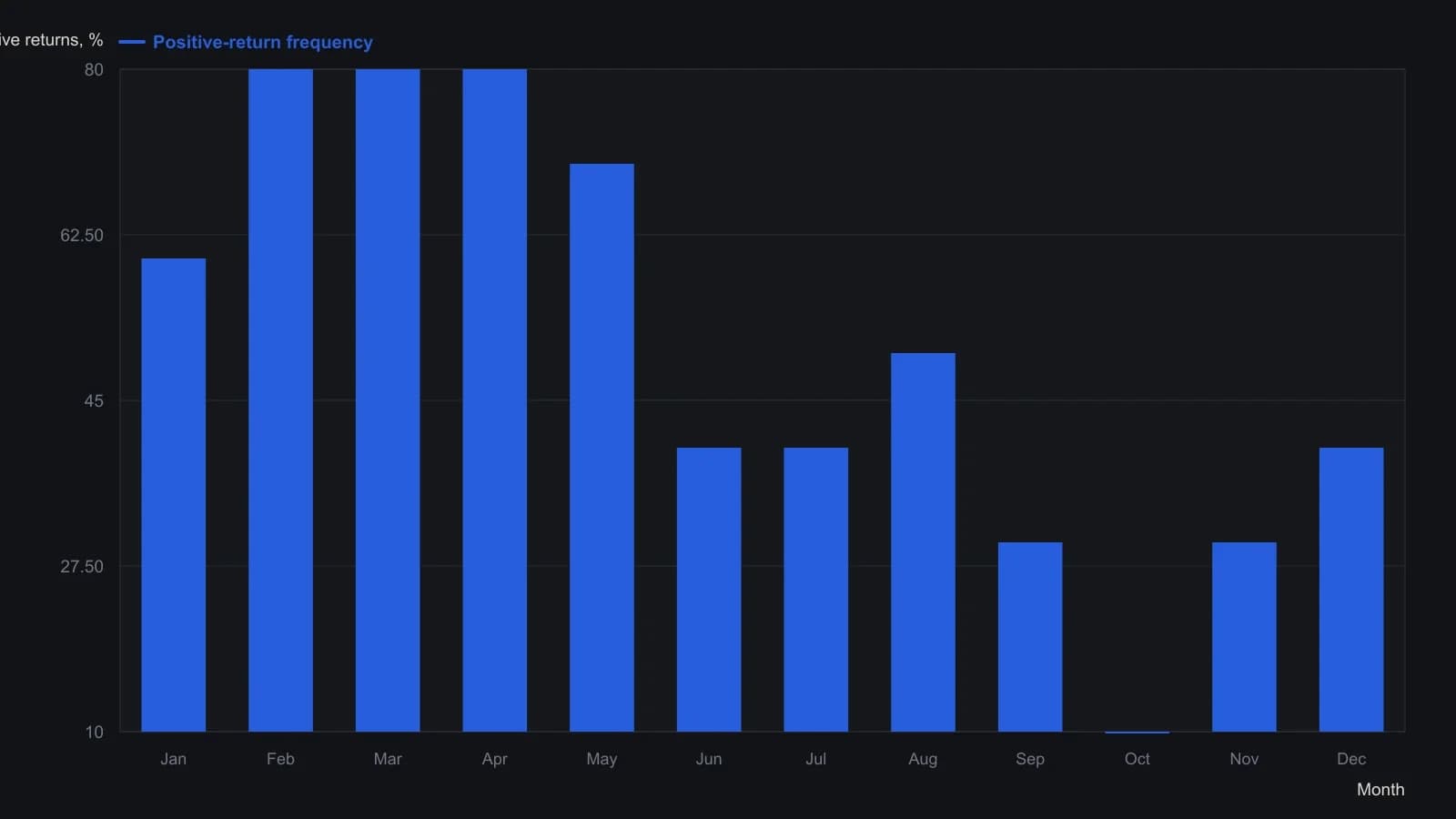
Each month’s price is divided by that year’s average, then 1 is subtracted. Frequency counts only the sign of that residual, not its size. The 2009–2018 window is the decade shown in the table.
A rolling four-year window and a consistency gate
The mechanical overlay averages each month’s positive-return frequency over the prior four years. That rolling four-year window recomputes monthly hit rates so the seasonal map can change as recent years replace older ones.
When two months tie at an extreme, the overlay uses the latest calendar month. It requires a high of at least 75 percent and a low of at most 25 percent before any trade is allowed. That pair of hit-rate thresholds is the consistency gate.
If the rolling frequency map is too muted to meet the consistency gate, the stance is seasonal abstention: stay flat.
Month-end calendar order
If the high-frequency month occurs first, the rule shorts at that month-end and covers at the low-frequency month-end. If the low-frequency month occurs first, it buys at that month-end and exits at the high-frequency month-end. Direction and holding span follow month-end calendar order: which extreme month arrives first in the year.
Movable equity calendars
Equity seasonality is treated as movable because shopping calendars, off-season travel discounts, and year-round retail can shift when monthly highs and lows appear. The same rule set is examined on commodity futures and on a narrow equity group of airlines, home builders, and large hotel chains.
A broad-market fund is used to show that a persistent upward drift can look like a seasonal edge if individual trades are not inspected.
A diversification sleeve
Because the frequency rules do not follow trend or momentum logic, they are framed as a diversification sleeve rather than a substitute for those approaches. In that framing the hit-rate map is a regime overlay: market-state context rather than a forecast of return size.
All readings on this track · 41 readings
- 1989Evaluating venue volume as a speculation-breadth signal
- 1991A thirty-name price-weighted average as a seasonal regime classroom
- 1991Ranked half-year rate changes as an equity signal filter
- 1991Demographic wave as a market-regime overlay
- 1994Seasonal range regimes as a futures context overlay
- 1996Evaluating presidential party terms as equity regimes
- 1996A dominant cycle is a baseline, not a reprint
- 1996Seasonality and presidential election cycle regimes
- 1997Stacking calendar regimes around election years
- 1997Calendar seasonality as a testable trading procedure
- 1997Lunar phase delay as a testable seasonal regime
- 1998Seasonal system construction without curve-fitting
- 1999Crowd life cycle as a market regime map
- 2001Regime-dependent cycle timing after four-year and seasonal lows
- 2002A 2002 case study in regime-first seasonal selection
- 2002Seasonal windows and dominant-cycle rules
- 2002Fifty-four-year wholesale cycle as an inflation-deflation regime map
- 2004The championship conference rule as a yearly regime case study
- 2004Election-year seasonality as trade regime context
- 2006Two-ten inversion as an intermarket regime filter
- 2006Midterm-to-presidential seasonal holding window
- 2008Two-layer equity regimes from seasonality and price history
- 2008Seasonal futures as a regime filter, not a calendar rule
- 2008Retesting seasonal rules when regimes change
- 2010Corn and wheat staggered calendars as dollar-neutral seasonal spreads
- 2011Name the S&P 500 trend regime before using weekly and monthly seasonality
- 2012Seasonal windows that wait for confirmation
- 2013Pair-sleeve rotation as a two-state sector regime-switch
- 2013Lunar phase as a seasonal overlay on implied volatility
- 2013Soybean seasonal highs in a five-year carryover regime
- 2014Year-end tax-loss selling as a seasonal regime
- 2017Calendar-window overlays that mute mechanical signals without rewriting the system
- 2017A four-year cycle and volume case study of a secular bear
- 2017Treat the valuation climate as climate and implied-volatility extremes as weather
- 2019Seasonal depth versus tracking for futures position sizing
- 2019Stacking cycle forecasts with seasonal regimes
- 2019Hit-rate gates for seasonal regime evaluation
- 2019July to October as a seasonal window, not a reason to own the name
- 2020A recession-regime checklist from valuation stretch and the yield curve
- 2020Treat a seasonal idea as a stay-or-sit holding procedure
- 2020A single position as a sleeve on a seasonal regime map