1995issue C091-7
Read one equity position on a joint yield-regime card
A half-year rate-change quintile plus a high, average, or low rate-level group turns a rates headline into a cell on a quantile grid, so one equity position is read in intermarket context.
- Intermarket analysis here places equity outcomes against contemporaneous long-term government-yield conditions instead of reading stock prices in isolation.
- The half-year sampling window pairs a 26-week yield lookback with a matching 26-week forward equity-price interval.
- Yield level was treated as a weak mapping on its own and became informative only inside a rate-change quintile, as a high, average, or low rate-level group.
- Editorially, a joint yield regime is a market-context state for a diversified book, not a standalone call on a single name.
Two axes instead of one headline
The archive paired each week with two half-year views of the long-term government yield: the direction of the recent move, and the altitude of the yield itself. Subsequent S&P 500 price change, dividends excluded, was then read against that pair.
Intermarket analysis, in this workflow, means placing those equity outcomes in the context of contemporaneous long-term government-yield conditions instead of reading stock prices in isolation.
The half-year sampling window
The half-year sampling window is a fixed 26-week lookback on yields paired with a matching 26-week forward equity-price interval. It is used as a repeating seasonal-length sampling unit.
The yield side is the prior 26-week continuously compounded percentage change in the long-term Treasury yield. That measure is then ranked, not treated as a one-line up or down label.
Rate-change quintiles and the weak level-only map
Those prior 26-week yield changes were ranked and split into five equal rate-change quintiles. Quintile 1 held the largest increases. Quintile 5 held the largest declines. The middle quintile collected the more stable-rate weeks.
A ranking by yield level alone was described as a weak mapping to subsequent equity returns. The level was treated as informative only when examined jointly with the recent change in yields.
S&P 500 average return by prior 26-week yield-change quintile
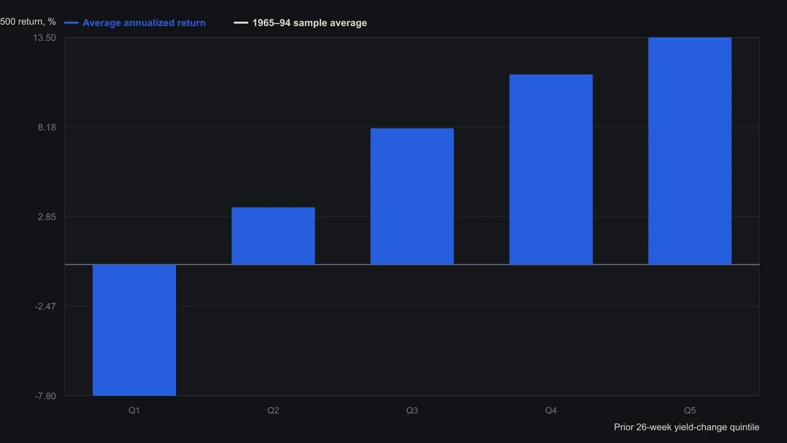
Equity returns are continuously compounded, exclude dividends, and are doubled to annualize. The yield is the 20-year Treasury through June 1977 and the 30-year thereafter. Q1 is the largest 20% of 26-week yield increases; Q5 is the largest 20% of declines.
Building the quantile grid
Inside each rate-change quintile, observations were re-ranked by the average of the current and 26-week-lagged long-term yield. That second rank was split into three equal rate-level groups: high, average, and low.
The quantile grid is the resulting two-way table. Each week is assigned a joint yield regime, which is the combined change-quintile and level-group label.
What the joint historical mapping showed
On that historical grid, attaching the rate-level group to a large-increase or large-decline rate-change quintile altered the subsequent 26-week equity-return description relative to the change quintile used alone. A sharp decline from a high yield level was associated with a stronger subsequent-return description than the same decline from a low yield level.
Except in the stable-rate middle quintile, the joint historical mapping was more favorable under high yield levels than under low yield levels. When yields were stable, subsequent equity outcomes were largely similar across high and low levels.
Two sample windows illustrated the extreme cells. One window showed high but rapidly falling yields coinciding with strong equity advances. Another showed low but rapidly rising yields, when the largest-increase rate-change quintile appeared on several occasions.
Robustness checks and an editorial reading
Suggested robustness checks included other yield instruments, other forward horizons, other change-lag lengths, a reversed rank order that sorts by level first, and closer attention to the most extreme tails of the joint distribution.
As a TradersWeek editorial reading, the joint yield regime is a market-context state for a diversified book, not a standalone call on a single name. Once both axes are filled in, one equity position is a cell on the quantile grid rather than a reaction to a single rates headline.
All readings on this track · 6 readings
- 1986Evaluate the price random-walk question as a gated quantile lab
- 1989Path quantiles versus net return for index velocity regimes
- 1992Opening-referenced percentile stops for same-session gaps
- 1995Read one equity position on a joint yield-regime card
- 2012Construct a pairs-trading worksheet from residuals and quantile ranks
- 2015Constructing mean, median, and mode from ordered prices