2006issue C041-4
Two-ten inversion as an intermarket regime filter
A 2006 two-ten snapshot is taught as a scored regime object. Curve shape, inversion depth and inversion duration come first, then policy-cycle position, and only then dollar carry, gold-linked crosses or growth risk.
- Classify the two-ten spread as a normal yield curve, a flat yield curve or an inverted yield curve before any portfolio story is allowed to change.
- Add inversion depth and inversion duration so a gap of a few basis points is not scored like a deep, sustained inversion.
- Use the inversion-to-recession lag as a multi-month timing window. Inversion has been a historical precondition for recession, not a sufficient trigger.
- Place the print in a policy-pause regime, then read carry-funding pairs and gold-linked crosses as portfolio context rather than as a first signal.
A print is not yet a regime
A two-ten print is easy to treat as a recession headline. This case study treats that print as a regime object that has to be scored before it is allowed to reframe anything else.
The editorial aim is layered confirmation rather than a single inversion banner. Map curve shape first. Time the print against the inversion-to-recession lag. Only then read cross-market prices as portfolio context for dollar carry, gold-linked crosses or growth risk.
Score shape, depth and duration first
A normal yield curve is the healthy case. Short-term yields sit below long-term yields, compensating investors for holding duration. An inverted yield curve is the reverse, when short-term yields exceed long-term yields, and is often read as a late-cycle or policy-tightening regime.
The two-ten spread, the gap between 10-year and two-year government yields, is the primary curve-shape classifier here. Inversion depth asks how far short-term yields exceed long-term yields. Inversion duration asks how long that state persists. Together they separate a brief wrinkle from a sustained regime.
The 2006 two-ten snapshot
At the 2006 snapshot the two-year yield was 4.60% and the 10-year yield was 4.31%, after the first two-ten inversion since 2000 appeared in the last week of December 2005. The contemporaneous gap was only a few basis points, and the curve was described as flatter than deeply inverted.
One stated reason investors accept a lower long-term yield is an expectation that growth has peaked, policy will tighten into that peak, and later easing will be required if the slowdown is deep. Depressed long-term US yields were also attributed to official Asian demand for Treasuries and to carry demand for dollar assets after US hikes, while Japanese policy rates remained at 0%.
A precondition, not a trigger
In the sample cited, each of the prior six recessions was preceded by a yield-curve inversion, with a typical lead of about 40 weeks. That inversion-to-recession lag is used here as a timing window rather than a calendar season. It places the print on a multi-month clock. It does not convert one inversion headline into a downturn date.
Inversion is treated as a historical precondition for recession, not a sufficient trigger. Two episodes in 45 years inverted without a recession: from the second quarter of 1966 through the first quarter of 1967, and from the third through fourth quarter of 1998.
Depth separates flat from historically deep
In that multi-decade record a recession was not observed unless the curve inverted by two percentage points or more. The 2006 gap was only a few basis points. Editorial reading: inversion depth is the filter that keeps a shallow flattening from being scored as a historically recession-linked inversion.
A flat curve was observed globally, not only in the United States, and was associated with a slower expansion pace. Average GDP growth in the referenced pattern eased from 4.2% the year before inversion to 2.3% the year after. A flat yield curve is therefore described as a slower-expansion regime rather than an automatic contraction.
Policy position after the curve is mapped
Across the plotted two-ten history, inversion has usually coincided with a pause or end to Federal Reserve hikes, including after 14 consecutive increases in the then-current cycle. That pattern is the policy-pause regime: the historical tendency for a hiking cycle to stall or end once the curve inverts.
Editorial reading: policy-cycle position is the third score on the object, after shape and after inversion depth and inversion duration. Until those layers are in place, the print is not ready to reframe growth risk.
Cross-market prices come last
Only after curve shape and policy-pause context are mapped should cross-market prices be read as portfolio context. In the five inversion windows tabulated, the dollar stayed flat or firmer against the yen and was mixed against the Swiss franc. That pattern is consistent with high short-term US rates, Japan’s sensitivity to global growth, and haven demand for gold-linked currencies when growth weakens.
The dollar against the yen sits here as a carry-funding pair: a high-yielding currency held against a low-yielding funder. The Swiss franc is treated as a gold-linked cross, a currency historically bid when growth anxiety lifts demand for gold as an alternate store of value. Editorial reading: those crosses may confirm or qualify the scored curve. They do not replace it.
Dollar returns across five yield-curve inversions
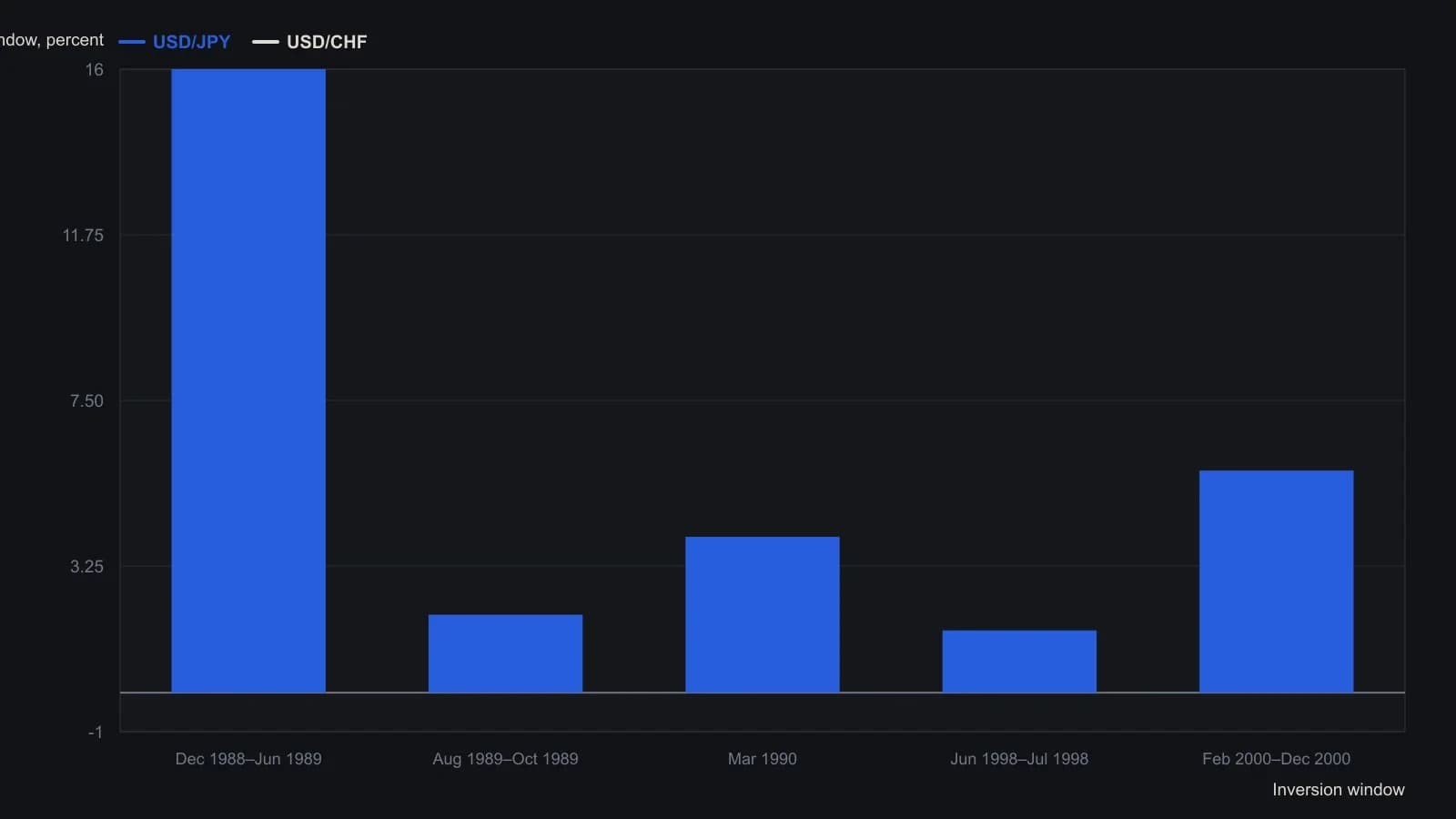
The source lists only these five inversion episodes as of the early-2006 writing and reports window returns, not start-to-end spot levels.
All readings on this track · 41 readings
- 1989Evaluating venue volume as a speculation-breadth signal
- 1991A thirty-name price-weighted average as a seasonal regime classroom
- 1991Ranked half-year rate changes as an equity signal filter
- 1991Demographic wave as a market-regime overlay
- 1994Seasonal range regimes as a futures context overlay
- 1996Evaluating presidential party terms as equity regimes
- 1996A dominant cycle is a baseline, not a reprint
- 1996Seasonality and presidential election cycle regimes
- 1997Stacking calendar regimes around election years
- 1997Calendar seasonality as a testable trading procedure
- 1997Lunar phase delay as a testable seasonal regime
- 1998Seasonal system construction without curve-fitting
- 1999Crowd life cycle as a market regime map
- 2001Regime-dependent cycle timing after four-year and seasonal lows
- 2002A 2002 case study in regime-first seasonal selection
- 2002Seasonal windows and dominant-cycle rules
- 2002Fifty-four-year wholesale cycle as an inflation-deflation regime map
- 2004The championship conference rule as a yearly regime case study
- 2004Election-year seasonality as trade regime context
- 2006Two-ten inversion as an intermarket regime filter
- 2006Midterm-to-presidential seasonal holding window
- 2008Two-layer equity regimes from seasonality and price history
- 2008Seasonal futures as a regime filter, not a calendar rule
- 2008Retesting seasonal rules when regimes change
- 2010Corn and wheat staggered calendars as dollar-neutral seasonal spreads
- 2011Name the S&P 500 trend regime before using weekly and monthly seasonality
- 2012Seasonal windows that wait for confirmation
- 2013Pair-sleeve rotation as a two-state sector regime-switch
- 2013Lunar phase as a seasonal overlay on implied volatility
- 2013Soybean seasonal highs in a five-year carryover regime
- 2014Year-end tax-loss selling as a seasonal regime
- 2017Calendar-window overlays that mute mechanical signals without rewriting the system
- 2017A four-year cycle and volume case study of a secular bear
- 2017Treat the valuation climate as climate and implied-volatility extremes as weather
- 2019Seasonal depth versus tracking for futures position sizing
- 2019Stacking cycle forecasts with seasonal regimes
- 2019Hit-rate gates for seasonal regime evaluation
- 2019July to October as a seasonal window, not a reason to own the name
- 2020A recession-regime checklist from valuation stretch and the yield curve
- 2020Treat a seasonal idea as a stay-or-sit holding procedure
- 2020A single position as a sleeve on a seasonal regime map