1991issue C051-7
A thirty-name price-weighted average as a seasonal regime classroom
Treat the familiar thirty-name industrial average as a regime classroom rather than a market census. Decode how composition-substitution and a shrinking divisor change what one point means, then place any single close against multi-decade volatility, dividend-multiples, and calendar-extremes so a seasonal or valuation reading can be tested as portfolio context.
- From October 1928 the printed series has been a thirty-name price-weighted average. Unadjusted closes were summed and divided by a divisor, first 16.67 rather than a weighted mean, later 0.505 after 63 years of splits, dividends, and substitutions.
- Composition-substitution is opaque and era-specific. One large technology name entered on May 26, 1932, left on March 14, 1939, and returned on June 29, 1979 after a 40-year absence.
- On July 16, 1990 the average closed at 2999.75. An extra 12.5 cents in one high-priced name would have printed 3000, yet only four names made 12-month highs and one large retailer printed a 12-month low.
- Editorial reading: dividend-multiples, yearly percent ranges, and calendar-extremes belong in a weeks-to-months market-regime that contextualizes a single trade, not as a standalone forecast.
A classroom, not a census
The familiar thirty-name industrial average dates from October 1928, when the roster was expanded from 20 stocks to 30. This editorial treats that printed series as a regime classroom, not as a market census.
Editorial framing uses seasonal analysis and seasonality analysis to put a single trade into a diversified or regime-aware context on a weeks-to-months horizon. Seasonal trading is reserved for making entry, exit, and abstention rules testable as one procedure over the system holding period.
How the printed average is built
Early construction added unadjusted closing prices and divided by the number of names. The 1928 version used a divisor of 16.67 rather than a weighted mean. In a price-weighted average, high-priced members move the printed level more than low-priced members.
After 63 years of splits, dividends, and substitutions the divisor had fallen from 16.67 to 0.505, so a small price change in any of the 30 names moves the published average by a much larger amount. Editorial reading: one point is not a stable unit of breadth. It is an artifact of the current divisor and of which names sit on the roster.
Roster changes as era markers
One large technology name entered the roster on May 26, 1932, left on March 14, 1939, and returned on June 29, 1979 after a 40-year absence. The archive presents that path as evidence that membership changes are opaque and era-specific.
This editorial treats composition-substitution as an era marker rather than a transparent, rules-based market definition. A seasonal or valuation reading taken from the printed average is a reading of the roster then in force, not of an unchanging industrial universe.
One close is not the roster
On July 16, 1990 the average closed at 2999.75. An extra 12.5 cents, or one-tenth of 1 percent, in one high-priced name would have printed 3000. Only four names made 12-month highs that day, and one large retailer printed a 12-month low.
Editorial reading: a round printed level can be a thin event. The close belongs next to how many names actually participated, not next to the integer alone.
Volatility, yield, and earnings multiples
Using each year’s percent range from low to high as a rough volatility gauge, only 1974 and 1987 among the prior 16 years approached the extremes of the early decades.
A common overvaluation shorthand of 30 times roster dividends, a 3-1/3 percent yield, sat near 3000 when 1990 dividends were about 100. A 75-year average dividend-multiple was 22.7 times dividends. The August 1987 yield of 2.6 percent was the lowest in 116 years.
From 1966 through 1982 the 1000 level repeatedly attracted approaches that failed to hold. The long earnings-multiple record shows the average can trade well below 10 times earnings before turning up. Editorial reading: those multiples and failed holds are regime context for a single trade, not a standalone forecast of the next move.
DJIA yearly high and low, 1960–1990
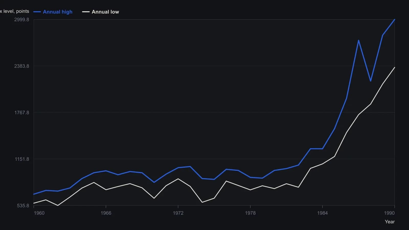
Points are the table’s annual Index Range High and Low columns, not year-end closes. The 1990 high is the July 16 close of 2999.75 discussed in the text; estimated 1990 earnings and dividend figures in the same table are unused here.
Month-of-year extremes
Across 63 years from 1928, August contained only one yearly high and one yearly low. October contained three highs and six lows. January and December hosted 28 and 25 yearly extremes. Nineteen yearly highs, 30 percent of the total, fell in December.
A calendar-extreme is only a count of years in which a given month contained that year’s high or low. Editorial reading: clustering of extremes is a market-regime overlay. It does not, by itself, generate an entry.
Test the reading as portfolio context
The editorial sequence is construction first, then membership, then one close against volatility, dividend-multiples, earnings multiples, and calendar-extremes. Seasonal analysis and seasonality analysis keep that stack in a weeks-to-months market-regime so a single trade sits in diversified or regime-aware context.
If the next step is a rule, seasonal trading folds entry, exit, and abstention into one testable procedure over the system holding period. This case study stops at the classroom: it does not state a trade.
All readings on this track · 41 readings
- 1989Evaluating venue volume as a speculation-breadth signal
- 1991A thirty-name price-weighted average as a seasonal regime classroom
- 1991Ranked half-year rate changes as an equity signal filter
- 1991Demographic wave as a market-regime overlay
- 1994Seasonal range regimes as a futures context overlay
- 1996Evaluating presidential party terms as equity regimes
- 1996A dominant cycle is a baseline, not a reprint
- 1996Seasonality and presidential election cycle regimes
- 1997Stacking calendar regimes around election years
- 1997Calendar seasonality as a testable trading procedure
- 1997Lunar phase delay as a testable seasonal regime
- 1998Seasonal system construction without curve-fitting
- 1999Crowd life cycle as a market regime map
- 2001Regime-dependent cycle timing after four-year and seasonal lows
- 2002A 2002 case study in regime-first seasonal selection
- 2002Seasonal windows and dominant-cycle rules
- 2002Fifty-four-year wholesale cycle as an inflation-deflation regime map
- 2004The championship conference rule as a yearly regime case study
- 2004Election-year seasonality as trade regime context
- 2006Two-ten inversion as an intermarket regime filter
- 2006Midterm-to-presidential seasonal holding window
- 2008Two-layer equity regimes from seasonality and price history
- 2008Seasonal futures as a regime filter, not a calendar rule
- 2008Retesting seasonal rules when regimes change
- 2010Corn and wheat staggered calendars as dollar-neutral seasonal spreads
- 2011Name the S&P 500 trend regime before using weekly and monthly seasonality
- 2012Seasonal windows that wait for confirmation
- 2013Pair-sleeve rotation as a two-state sector regime-switch
- 2013Lunar phase as a seasonal overlay on implied volatility
- 2013Soybean seasonal highs in a five-year carryover regime
- 2014Year-end tax-loss selling as a seasonal regime
- 2017Calendar-window overlays that mute mechanical signals without rewriting the system
- 2017A four-year cycle and volume case study of a secular bear
- 2017Treat the valuation climate as climate and implied-volatility extremes as weather
- 2019Seasonal depth versus tracking for futures position sizing
- 2019Stacking cycle forecasts with seasonal regimes
- 2019Hit-rate gates for seasonal regime evaluation
- 2019July to October as a seasonal window, not a reason to own the name
- 2020A recession-regime checklist from valuation stretch and the yield curve
- 2020Treat a seasonal idea as a stay-or-sit holding procedure
- 2020A single position as a sleeve on a seasonal regime map