1991issue C081-12
Name the window, then combine leaders
Name an exact calendar window, rank current leaders with a two-series linear-regression screen, drop mid-range seasonal links, and only then average the surviving force series into one forecast screen.
- The correlation coefficient between Treasury bonds and a broad equity index changes with every span from 3 days to 300 days, so the calendar window has to be named before any combination is built.
- A linear-regression screen favors a direct scale when the coefficient sits between +0.5 and +1.0, an inverse scale between -0.5 and -1.0, and sets a mid-range series aside for that window.
- Force series keep reversal dates in place. A 20-day moving average adds a 10-day lag and can erase a leader whose initial lead is only about five days.
- Re-rank the weighted combination when the seasonal sample changes. A frozen favorite mixes windows where that series is strong with windows where it is weak.
Name the calendar window first
The archive workflow builds a combination only after a calendar window is named. A two-column linear-regression screen then ranks which leading indicators currently lead a target, mid-range series are set aside, and the surviving force series are averaged into one composite leading index.
The association between Treasury bonds and a broad equity index is not one number. Recomputing it for every span from 3 days to 300 days produces a different correlation coefficient for each exact horizon. The same bond-equity pair can imply opposite lead stories when one chart covers a short seasonal slice such as May 1987 and another covers the longer overlapping stretch of the first nine months of 1987.
A calendar window is the exact day count and date range that define one seasonal or regime sample. Changing it can reverse the apparent lead, so the window is stated before any ranking begins.
Rank candidates with a linear-regression screen
Scale direction for a candidate leader can be chosen from a two-column linear regression. A correlation coefficient between +0.5 and +1.0 favors a direct scale. A coefficient between -0.5 and -1.0 favors an inverse scale. A mid-range result is a reason to set that series aside for the current window.
That linear-regression screen decides scale direction and ranks candidate leaders before any composite is built. A leading indicator is a market or economic series whose turns are tested as arriving before those of a target index inside the named window.
Rescale into force series
A force series is an affine rescaling of a raw indicator so several series can share a chart with the target without moving reversal dates. Converting raw indicators into comparable force series with an additive and a multiplicative constant changes chart placement and pattern geometry but leaves the calendar dates of reversals unchanged, unlike a moving average that adds lag.
A 20-day moving average introduces a 10-day lag, which can erase a leader whose initial lead is only about five days. Lagging smoothers are a poor substitute for force rescaling.
Leader rank is period-specific
Leader rank belongs to one period, not to a permanent favorite. In 1973-74 one large-cap share price fell 60% while its earnings rose 45%, so earnings were a weak leader then. An inversely scaled oil force later showed a 0.839 correlation with the equity index between 1 October 1990 and 1 February 1991.
Keeping the same favorite indicator through every calendar regime mixes windows where that series is strong with windows where it is weak. A combination must be re-ranked when the seasonal sample changes rather than frozen as a permanent leader.
Average only the surviving forces
A combination built for a named window ranks candidate forces by current regression strength, converts them to a common scale, assigns weights that sum to 10, and averages those weighted forces into one composite leading index.
A second composite that puts more weight on the largest forces can be paired with the first. A line joining their successive turns points toward a later target turn and begins to appear about 2 to 20 days before that turn. The pair is a preliminary screen rather than a lagging crossover. That second series is a secondary guide index, with turns that fall between the first composite and the target.
Date the buy and sell zones
A combined screen can be audited by dating each buy zone and sell zone, growing a theoretical book with the equity benchmark in buy zones and an 8% annual cash rate in sell zones, then comparing that path with the benchmark and counting the share of profitable zones.
A buy zone is a dated interval when the combined screen treats the target as aligned with a benchmark-linked book. A sell zone is a dated interval when the same screen parks the book in a stated cash-rate placeholder.
IBM earnings rose while the share price fell, 1973–74
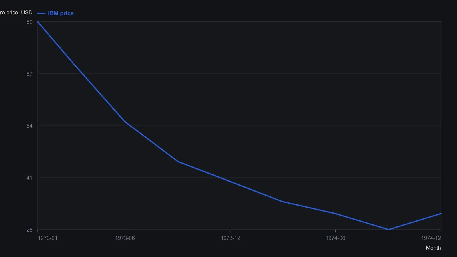
Approximate digitization of the printed Figure 3 raster; the source states a 60 percent price drop against a 45 percent earnings rise and does not print a numeric table.
All readings on this track · 37 readings
- 1988Constructing a lead-aware correlation coefficient
- 1989A precious-metal price as a changing intermarket equation
- 1990Two clocks for copper: a factor regime, a regression baseline, and leftover moving-average timing
- 1990Earnings yield, rate correlation and regression for equity value
- 1991Name the window, then combine leaders
- 1991Constructing a two-market linear correlation check
- 1991Constructing a commodity-bond correlation regime filter
- 1992Building intermarket context with linear correlation
- 1993Inverse-scale overlays as a gold-equity regime filter
- 1994Constructing seasonal slots from windows, analog years, and implied volatility
- 1995Pin one reference close and roll companion correlations as an overlay
- 1995Rolling correlation windows for shifting intermarket regimes
- 1998Gold as a cross-market regime barometer
- 1999The gold-bond inverse is a regime, not a cause
- 1999A nested lag test of gold leading bond yields
- 1999Constructing spreads from stock and intermarket correlation
- 2000Evaluating headline versus food-and-energy-excluded CPI as bond-yield context
- 2005A late EUR/USD fifth wave tested by the Bund-Treasury gap
- 2006Intermarket dislocation as context for short-horizon momentum
- 2008Map ordinary 12-month outcomes before stacking valuation, rates, and seasonality
- 2008A clean-energy theme inside the oil-and-energy regime
- 2014Quantitative-easing overlays as fragile belief regimes
- 2015Three intermarket checks from the late-2014 crude decline
- 2015Basket construction via rank, correlation, and locked rules
- 2015Construct a CAD-oil pair from percent-of-range Bollinger maps
- 2015CAD/USD and crude: first the correlation, then the band gap
- 2017Correlation regime versus moving-average crossover for S&P 500 exposure
- 2017Updating intermarket systems after correlation shifts
- 2017Constructing a correlation-divergence regime filter for yen and Nikkei context
- 2018Clustered negative troughs in an energy-index pairwise correlation
- 2018Filter pairwise-correlation before reading an intermarket regime
- 2018Moving-average supports in the March 2018 correlation shock
- 2020Bond spreads as an equity regime lens
- 2020Crash-protection folklore as a correlation regime question
- 2020Constructing a bounded correlation-trend-filter
- 2020Constructing a correlation-to-line trend filter
- 2020Bitcoin correlation regimes across equities and gold