1991issue C121
Constructing a two-market linear correlation check
A short intermarket construction pairs two closes under a straight-line association check, then reads the coefficient as portfolio context rather than a causal story or lead-lag forecast.
- An intermarket pair is built by assigning two market closes as X and Y and imposing a linear baseline before a single trade is read in a diversified book.
- The correlation coefficient is bounded between +1 and -1, with 0 marking no linear association, and it does not index curved relationships.
- A large positive coefficient measures co-movement only and does not show that one series produces the other.
- The supplied construction uses ten paired observations of bond-futures and commodity-index closes and produces a coefficient of 0.83.
This archive article reconstructs a small intermarket construction: treat two markets as a paired check, impose a linear baseline, and read the resulting correlation coefficient as context for how tightly those series are moving together. The aim is not a causal story and not a lead-lag forecast.
Editorial reading: use the coefficient to place one intended position against a second market before the book is treated as diversified or regime-aware.
What the coefficient measures
An intermarket pair assigns two distinct market series as X and Y so one position can be checked against a second market. The linear baseline is the modeling assumption that the paired series can be described by a straight line when one is plotted against the other.
The correlation coefficient is a bounded index of linear association between two series. It runs from a perfect inverse reading through no linear association to a perfect positive reading. In plain bounds, the index sits between +1 and -1, and 0 indicates no linear association.
Because the index is restricted to straight-line relationships, it is not the correct measure when the paired series follow a curve.
Association is not causation
Association-versus-causation is the rule that a large coefficient measures co-movement only and does not show that one series produces the other. A large positive coefficient does not establish that a high reading in one series causes a high reading in the other.
Editorial reading: treat the finished number as a tightness check on the intermarket pair, not as proof that one market drives the other.
The ten-observation construction
The observation window is the count of paired closes used to assemble the coefficient. The supplied construction uses ten observations, a count presented as unusually small.
The worked construction assigns bond-futures closes as the X series and a commodity-price-index close as the Y series. Over that ten-observation window the worksheet produces a coefficient of 0.83 from a numerator of -12.87 and a denominator of 15.57. The same window has a mean bond-futures close of 94.15 and a mean commodity-index close of 219.99.
How to read the finished check
Editorial reading: once the coefficient is in hand, the intermarket pair functions as a constructed linear baseline that can sit beside a single trade idea. The coefficient says how tightly the two closes moved together inside the observation window. It does not by itself rank the trade, time an entry, or replace the rest of a diversified or regime-aware process.
Bond futures and CRB closes in the ten-day worksheet
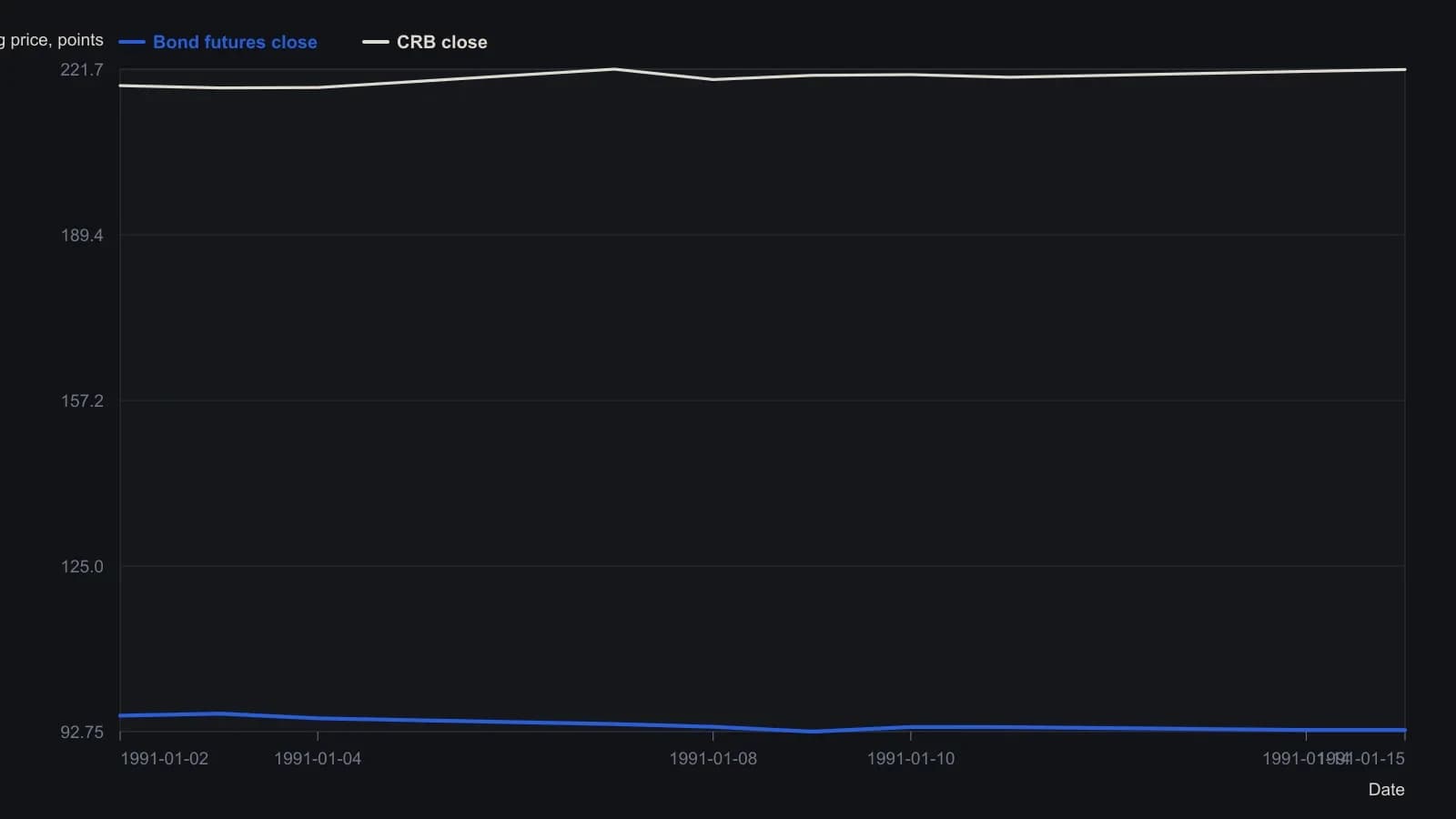
The source locked the window at n = 10 and said that sample is too small, a space limit rather than a working lookback. Only the linear formula is applied.
All readings on this track · 37 readings
- 1988Constructing a lead-aware correlation coefficient
- 1989A precious-metal price as a changing intermarket equation
- 1990Two clocks for copper: a factor regime, a regression baseline, and leftover moving-average timing
- 1990Earnings yield, rate correlation and regression for equity value
- 1991Name the window, then combine leaders
- 1991Constructing a two-market linear correlation check
- 1991Constructing a commodity-bond correlation regime filter
- 1992Building intermarket context with linear correlation
- 1993Inverse-scale overlays as a gold-equity regime filter
- 1994Constructing seasonal slots from windows, analog years, and implied volatility
- 1995Pin one reference close and roll companion correlations as an overlay
- 1995Rolling correlation windows for shifting intermarket regimes
- 1998Gold as a cross-market regime barometer
- 1999The gold-bond inverse is a regime, not a cause
- 1999A nested lag test of gold leading bond yields
- 1999Constructing spreads from stock and intermarket correlation
- 2000Evaluating headline versus food-and-energy-excluded CPI as bond-yield context
- 2005A late EUR/USD fifth wave tested by the Bund-Treasury gap
- 2006Intermarket dislocation as context for short-horizon momentum
- 2008Map ordinary 12-month outcomes before stacking valuation, rates, and seasonality
- 2008A clean-energy theme inside the oil-and-energy regime
- 2014Quantitative-easing overlays as fragile belief regimes
- 2015Three intermarket checks from the late-2014 crude decline
- 2015Basket construction via rank, correlation, and locked rules
- 2015Construct a CAD-oil pair from percent-of-range Bollinger maps
- 2015CAD/USD and crude: first the correlation, then the band gap
- 2017Correlation regime versus moving-average crossover for S&P 500 exposure
- 2017Updating intermarket systems after correlation shifts
- 2017Constructing a correlation-divergence regime filter for yen and Nikkei context
- 2018Clustered negative troughs in an energy-index pairwise correlation
- 2018Filter pairwise-correlation before reading an intermarket regime
- 2018Moving-average supports in the March 2018 correlation shock
- 2020Bond spreads as an equity regime lens
- 2020Crash-protection folklore as a correlation regime question
- 2020Constructing a bounded correlation-trend-filter
- 2020Constructing a correlation-to-line trend filter
- 2020Bitcoin correlation regimes across equities and gold