2018issue C0120-23
Clustered negative troughs in an energy-index pairwise correlation
A 13-week energy-versus-index pairwise-correlation averaged 0.63 and stayed positive overall. The case study treated clustered-negative-troughs, a spacing-filter, and a recovery-clock as one procedure, including when to stand aside.
- The energy-versus-index pairwise-correlation averaged 0.63 with a standard deviation of 0.34, remained positive overall, and did not line up one-for-one with the index close.
- Clustered-negative-troughs fewer than 25 weeks apart were recorded as later index-top cases. Two wider-spaced pairs were recorded as false positives under the spacing-filter.
- A recovery-clock measured the index's largest decline over the next 52 weeks from the second trough, the later zero cross, or the later 0.5 cross.
- The setup was one procedure with regime-abstention when the troughs were more than 25 weeks apart. The March-June 2017 path was treated as outside the earlier sample pattern.
A positive average that is still only context
The study built a 13-week pairwise-correlation from weekly adjusted closes of an energy-sector fund and a broad S&P 500 fund. The pair was one case in a sector-by-sector series.
On the plotted history that pairwise-correlation averaged 0.63 with a standard deviation of 0.34 and remained positive overall. Its level did not line up one-for-one with the index close.
Clustered negative troughs and the spacing filter
Selected episodes with two negative correlation troughs fewer than 25 weeks apart were aligned with later index peaks and subsequent declines. Those clustered-negative-troughs included 2000, 2006-2007, and 2014.
Every pair of negative troughs less than 52 weeks apart from January 2000 through June 2017 was collected. Seven paired-trough events entered that table. The five with troughs fewer than 25 weeks apart were recorded as later index-top cases. The two with wider spacing were recorded as false positives under the spacing-filter.
Three recovery clocks on a 52-week window
The index's largest decline over the next 52 weeks was measured from three recovery-clock starts: the second trough, the later move through zero, and the later move through 0.5.
When the two troughs were 25 weeks or closer, the tabulated average 52-week maximum index declines were 12.8% from the second trough, 11.5% from the later zero cross, and 14.1% from the later 0.5 cross. The two wider-spaced cases averaged 0.0%, 0.6%, and 1.9% on the same clocks.
S&P 500 max drop after clustered XLE/SPY correlation troughs
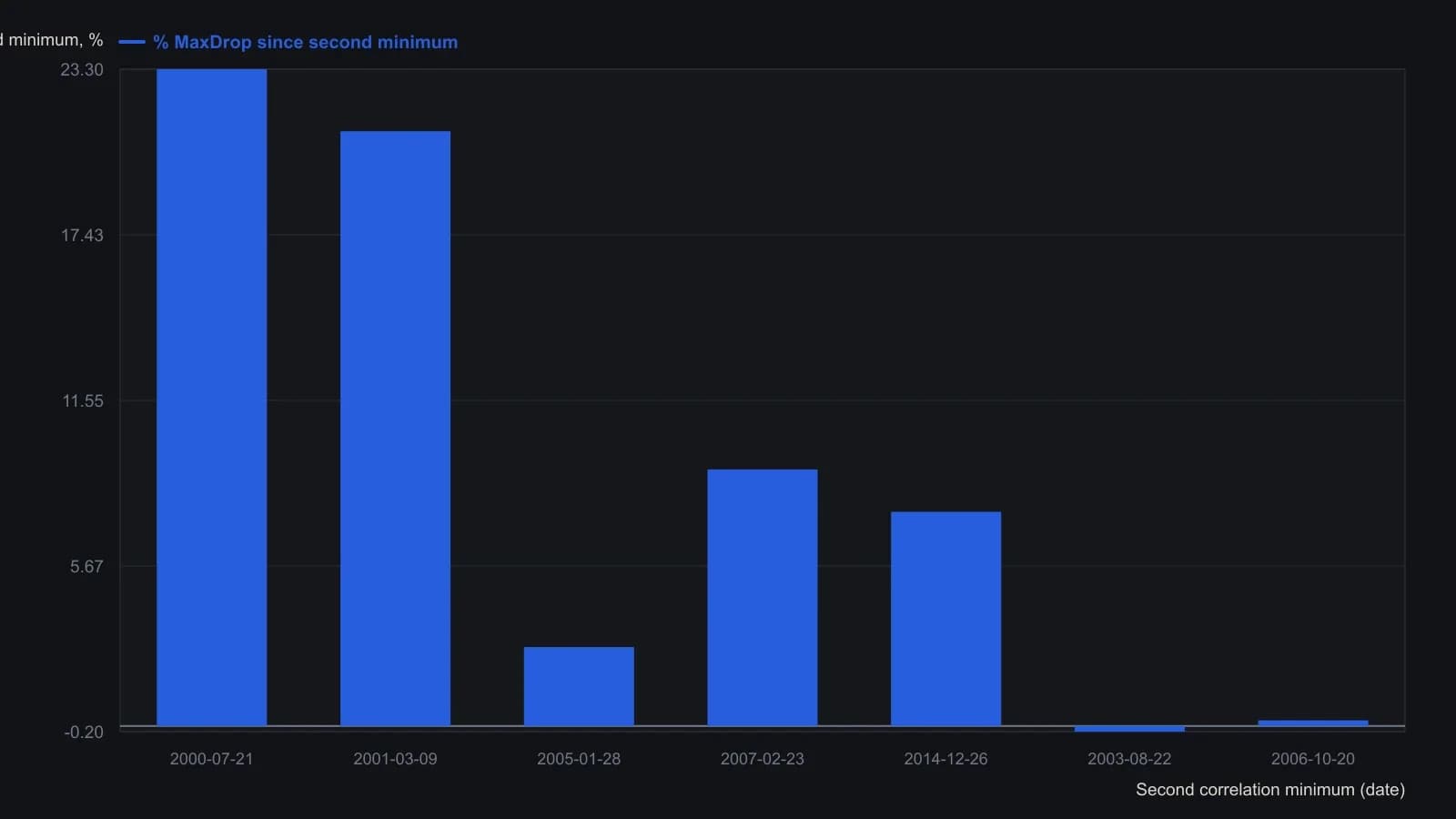
MaxDrop is the largest S&P 500 close-price decline in the 52 weeks after the second negative correlation minimum. Rows 1–5 are the under-25-week cluster; rows 6–7 exceed 25 weeks and were treated as false positives.
One procedure and a path outside the sample
The write-up specified the setup as one procedure with a chosen recovery-clock, a 52-week observation window, and abstention when the two negative troughs were more than 25 weeks apart.
From March through June 2017 the same series printed two deep negative troughs, including a reading of -0.934 on 17 March 2017 described as an 18-year low, without first recovering through zero. That path was treated as outside the earlier sample pattern.
All readings on this track · 37 readings
- 1988Constructing a lead-aware correlation coefficient
- 1989A precious-metal price as a changing intermarket equation
- 1990Two clocks for copper: a factor regime, a regression baseline, and leftover moving-average timing
- 1990Earnings yield, rate correlation and regression for equity value
- 1991Name the window, then combine leaders
- 1991Constructing a two-market linear correlation check
- 1991Constructing a commodity-bond correlation regime filter
- 1992Building intermarket context with linear correlation
- 1993Inverse-scale overlays as a gold-equity regime filter
- 1994Constructing seasonal slots from windows, analog years, and implied volatility
- 1995Pin one reference close and roll companion correlations as an overlay
- 1995Rolling correlation windows for shifting intermarket regimes
- 1998Gold as a cross-market regime barometer
- 1999The gold-bond inverse is a regime, not a cause
- 1999A nested lag test of gold leading bond yields
- 1999Constructing spreads from stock and intermarket correlation
- 2000Evaluating headline versus food-and-energy-excluded CPI as bond-yield context
- 2005A late EUR/USD fifth wave tested by the Bund-Treasury gap
- 2006Intermarket dislocation as context for short-horizon momentum
- 2008Map ordinary 12-month outcomes before stacking valuation, rates, and seasonality
- 2008A clean-energy theme inside the oil-and-energy regime
- 2014Quantitative-easing overlays as fragile belief regimes
- 2015Three intermarket checks from the late-2014 crude decline
- 2015Basket construction via rank, correlation, and locked rules
- 2015Construct a CAD-oil pair from percent-of-range Bollinger maps
- 2015CAD/USD and crude: first the correlation, then the band gap
- 2017Correlation regime versus moving-average crossover for S&P 500 exposure
- 2017Updating intermarket systems after correlation shifts
- 2017Constructing a correlation-divergence regime filter for yen and Nikkei context
- 2018Clustered negative troughs in an energy-index pairwise correlation
- 2018Filter pairwise-correlation before reading an intermarket regime
- 2018Moving-average supports in the March 2018 correlation shock
- 2020Bond spreads as an equity regime lens
- 2020Crash-protection folklore as a correlation regime question
- 2020Constructing a bounded correlation-trend-filter
- 2020Constructing a correlation-to-line trend filter
- 2020Bitcoin correlation regimes across equities and gold