2007issue C111-3

Constructing commodity seasonal indexes for regime context

A seasonal index is first a percentage map of typical price location across a fixed sample window. Only after that map is built does the archive scale a later seasonal leg for a larger realized move, then let a double-top measurement independently mark where the cycle may fail.

A seasonal index is built by averaging prices over a chosen day, week, or month window and stating each interval as an index rating against the full-window average.
Agricultural indexes can use a marketing year so harvest weakness and planting strength sit in the correct windows.
A volatility-scaled projection sizes a later seasonal leg from the ratio of a recent realized move to the typical earlier-leg move.
A double-top measurement is a separate downside check, and peaks or troughs are expected inside a seasonal window rather than on a required date.

Entries in this reading3 entries

Seasonality analysis24 readings Seasonal trading60 readings Current trackDouble top and bottom68 readings

Commodity cycles as a percentage map

Commodity markets are described as having calendar-year supply-and-demand cycles, with grains typically weakest near harvest and strongest during planting.

A seasonal index turns that cycle into a percentage map of typical price location by interval. It is formed by dividing each interval average by the average of all intervals in the sample.

Fix the sample, then rate each interval

The construction step is to average prices over a chosen day, week, or month window and rate each interval as a percentage of the full-window average. That rating is the index rating: an interval average expressed as a percent of the full-sample average, so readings below 100 mark historically weak windows and readings above 100 mark historically strong windows.

Agricultural series need not follow the calendar. A marketing year is a crop-aligned year used instead of the calendar year when building an agricultural index, here June through the following May for Chicago wheat.

Chicago wheat five-year seasonal index

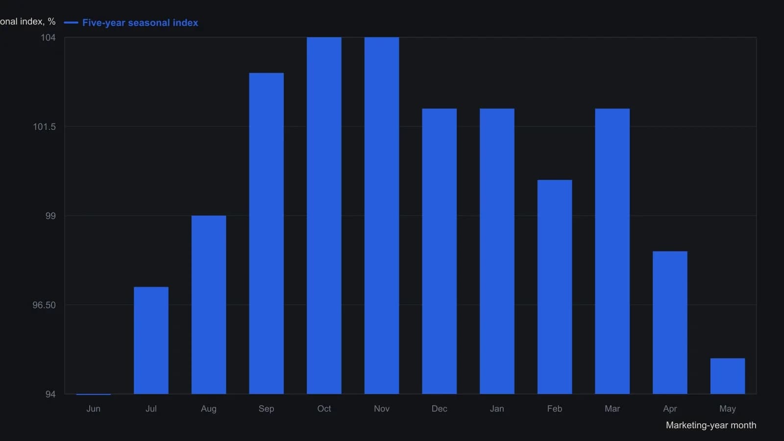
Harvest months sit near 94–95 percent of the five-year mean and the map peaks at 104 percent in October–November, so the regime is a harvest low and a planting-season high rather than a day-specific target. The points are the article’s table of monthly front-month averages divided by the $3.10 yearly mean.Chicago wheat front-month futures · monthly

The source fixes a five-year window of monthly front-month closes and a June–May marketing year. June and May both print a $2.93 average close, yet the table rates them 94 percent and 95 percent; those printed ratings are carried as given.

Wheat and gasoline maps from a five-year window

A five-year Chicago wheat index using marketing-year monthly closes from June through May rated June at 94 percent of the 3.10 yearly average and November at 104 percent.

A five-year weekly gasoline index for 2002 through 2006 placed the typical trough near 85 percent in mid-February and the typical peak near 112 percent in mid-August.

When a recent leg outruns the index

An early-2006 gasoline rise of about 50 percent was compared with a typical 22 percent index rise. The resulting 2.22-to-1 ratio was applied to a later seasonal leg the index marked at about 13 percent.

That step is a volatility-scaled projection: a later seasonal-leg magnitude obtained by multiplying the typical index percentage change by the ratio of a recent realized move to the typical move on the earlier leg. Applying that scaled later-leg percentage to a late-April cash print of 2.1374 produced a summer-peak figure of about 3.55.

A double top as a separate measure

Cash gasoline then formed a double top near 3.40 with an intervening trough near 2.90. Falling volatility was cited as the reason the later advance stopped short of 3.55.

A double-top measurement takes a downside objective from two similar highs and the trough between them, then subtracts that height from the trough. Subtracting the double-top height of 0.50 from the 2.90 trough produced a later-cycle low estimate of about 2.40, aligned with the seasonal decline window from mid-August through mid-February.

Structure can persist inside a seasonal window

A five-year crude-oil seasonal index continued to track front-month futures after open interest had nearly doubled since 2005, contrary to the argument that electronic and long-only fund flow would erase seasonal structure.

Seasonal indexes are framed as approximate guides, with peaks and troughs allowed to arrive inside a time window rather than on a fixed day, week, or month. A seasonal window is a rough span of weeks in which a seasonal peak or trough is expected, rather than a single required date.

Educational research material, not investment advice. Historical source context does not establish present-day performance.

23 of 32 in the Double top and bottom track

20091-69 pp.Next on Double top and bottomConstructing rounded and double-top short setupsLock the cup first as a saucer, oval, or inverted-V topping outline on OHLC before any handle is drawn.

All readings on this track · 32 readings

By fieldSeasonality and regimes93 readings By year200773 readings

All 68 readings tagged Double top and bottom

Also on Double top and bottom5 readings

1989Weekday price paths are regime-dependentSeasonality analysis 1990Calendar windows as testable index-futures proceduresSeasonality analysis 1996Nested calendar clocks in long-bond futuresSeasonality analysis 2008The January effect as a short window versus the monthSeasonality analysis 2013Calendar seasonality as a regime filter, not a standalone signalSeasonality analysis