1984issue C041-19
How to construct a maximum-entropy cycle model
A maximum-entropy fit can resolve dominant cycles from a relatively short ordered series, and the same coefficients can later produce a forecast consistent with those cycles. Construction starts with lookback and sample interval, a decision on data differencing, and order selection by final prediction error. Spectral analysis then turns those coefficients into power or amplitude so the peaks can be checked.
- Start with sixty to one hundred twenty observations, and prefer a series that covers at least the longest cycle of interest.
- Skip data differencing unless the goal is a momentum-style forecast or the optimizer flags it.
- In automatic mode, search order and sample interval with final prediction error, then keep the last-pass order if that rerun at the stored optimum is smaller.
- Treat a single broad peak at order one or two, an error minimum at the largest allowed order, or several local minima as a reason to revise the window, sample interval, or differencing choice.
What the fit produces
A maximum-entropy spectrum is a high-resolution spectrum estimated from a short ordered series by fitting coefficients that can later drive a cycle-consistent forecast. The same coefficients that resolve dominant cycles can later produce a forecast consistent with those cycles.
Spectral analysis converts those fitted coefficients into power or amplitude versus frequency or cycle length so peaks can be compared and the model checked. The dominant cycle is the strongest periodic component identified in the fitted spectrum, and it is used to judge whether the selected order and sample interval resolved a usable cycle.
Choose lookback and sample interval
Sixty to one hundred twenty observations are a practical starting lookback, and the series should ideally cover at least the longest cycle of interest.
The sample interval is the smoothing-and-resampling stride applied before the fit. Changing the sample interval shortens the plotted frequency range by the reciprocal of that interval and can move peak locations, so spectra from different intervals are not directly overlaid.
Decide whether to difference
Data differencing replaces each observation with its change from the prior bar to weaken a long trend when momentum, not level, is the intended input. Differencing is mainly for momentum-style forecasts and should be skipped unless that is the goal or the optimizer flags it.
Pick order with final prediction error
Automatic mode searches order and sample interval with a final-prediction-error criterion, while manual mode lets the user set coefficient length and the moving-average resample stride. Final prediction error is the order-selection score computed at each fit iteration, and the minimizing order is the recommended model length.
In automatic mode the fit is repeated for sample intervals one through five, then rerun at the stored optimum. If the last pass picks a smaller order, that last-pass order is the one recommended for spectrum work and forecasting.
Final prediction error by MEM order
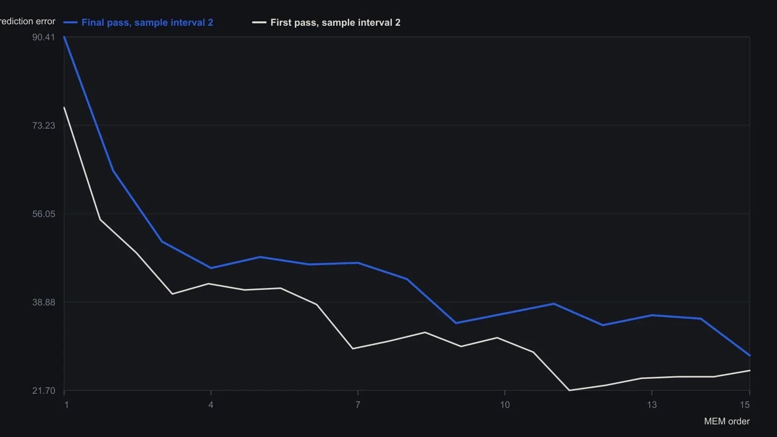
Auto mode scanned sample intervals D=1 through 5. Each printer plot marks the FPE minimum with a plus. The last pass used the optimized order M=15 rather than the longest order tried on the first D=2 pass.
Convert coefficients into a spectrum
Spectrum output may use log power from 0 to -40 dB or linear amplitude, with frequency in cycles per day preferred over cycle length. Values between -20 and -40 dB are only marginally significant.
Revise a bad window
A minimizing order of one or two yields a single broad peak and usually means a bad window, too large a sample interval, or a strong trend in noisy data, so the lookback or differencing choice should be revised.
If the error minimum sits at the largest allowed order or the error curve has several local minima, the series is too short or too little smoothing was applied. Lengthen the window toward at least three times sample interval times order when possible.
What remains after the plot
Fitted coefficients are stored with the spectrum values and remain available after the plot. The implementation is a computational subroutine that expects a user-supplied price-volume matrix rather than its own data feed or graphics.
All readings on this track · 28 readings
- 1984Constructing maximum-entropy spectra for dominant-cycle forecasts
- 1984How to construct a maximum-entropy cycle model
- 1984Constructing a maximum-entropy forecast from a chosen lookback
- 1985Constructing period-locked half-cycle and full-cycle averages
- 1986Why Fourier windows limit dominant-cycle resolution
- 1987Assembling short-lookback maximum-entropy cycle forecasts
- 1988Why a fitted dominant cycle is not a forecast
- 1989Evaluating commodity cycle personalities with spectral histograms
- 1989Evaluating next-session cycle forecasts with stops
- 1989Constructing cycle-aged volatility trailing stops
- 1990A channel signal-to-noise gate for dominant-cycle forecasts
- 1990Year-over-year dominant cycle personality audit
- 1991Cyclic entry from a locked dominant-cycle phase
- 1992Stationarity states on synchronized futures spectral contours
- 1997Hidden horizon assumptions in dominant-cycle readings
- 1997When market cycles are absent more than present
- 1997A spectral estimator that retunes indicators to the measured cycle
- 2000Constructing a Hilbert dominant cycle and a maximum-entropy refinement
- 2000Switch trend and cycle indicators after a half-cycle dwell test
- 2000Constructing a dominant-cycle squelch trend filter
- 2000Phasor displays for dominant-cycle construction
- 2002Low-lag trendline from elliptic and dominant-cycle notches
- 2004Spectral peaks are mode diagnostics, not forecasts
- 2004Compressive last-stage oscillator construction
- 2013Constructing trend failure curves from qualified-trend transitions
- 2014Lookback range, a two-lag smoother, and next-bar fills
- 2014Constructing a MESA stochastic with roofing and SuperSmoother filters
- 2016Constructing spectral heatmaps for dominant market cycles