1984issue C011-10
Constructing maximum-entropy spectra for dominant-cycle forecasts
A maximum-entropy spectrum is built from a linear predictor so later short-horizon forecasts stay consistent with the dominant-cycle peaks. Construction means choosing model order, auditing those peaks against Fourier analysis, and discarding interference before a forecast is allowed to inherit the cycle.
- The same linear predictor both estimates the data spectrum and generates adaptive short-horizon forecasts that must stay consistent with dominant-cycle peaks.
- Model order is the central construction choice because the number of spectral peaks is about half the coefficient count: too small an order misses cycles, and too large an order can add peaks that are not in the observations.
- Fourier analysis is the construction check on peak location. For forecasting, only the lowest-frequency peaks near the dominant cycle, those within 15 dB, are treated as signal.
- When extra peaks appear, the constructor can keep a local final-prediction-error minimum or average samples so the retained spectrum keeps the dominant-cycle shape with fewer noise peaks.
Two jobs in one construction
The method is constructed to serve two jobs at once: estimate a data spectrum and generate adaptive short-horizon forecasts that stay consistent with the dominant cycles found as spectral peaks.
A maximum-entropy spectrum is a spectrum built from linear-prediction coefficients chosen to minimize forecast error while adding as little extra structure as possible to the observed series. The dominant cycle is the strongest low-frequency spectral peaks retained as the signal that later forecasts and filter lengths are required to follow.
A linear predictor as the shared engine
Construction assumes the current observation equals a linear combination of M past values plus a residual. The coefficients are chosen to minimize squared prediction error and, in the usual algorithms, the sum of forward and backward residuals.
After the coefficients are fit, the spectrum is computed from those coefficients. Multi-step forecasts are formed recursively by feeding earlier predictions back into the same linear predictor.
Trend channels around the point forecast
A trend channel is the upper and lower bands around a recursive point forecast. The bands are built by adding and subtracting twice the square root of the n-step forecast-error variance around the point forecast, described as a 95 percent interval. Preprocessing used to quiet trading noise adds a further variance term.
Model order as the main design choice
Model order is the number of lagged coefficients in the predictor. The number of spectral peaks is about half the coefficient count, so the choice controls both resolution and the risk of spurious peaks.
Too small an order misses cycles. Too large an order can add peaks that are not in the observations.
Scoring candidate orders
Orders from 1 up to the smaller of half the sample length or 25 are scored with a final prediction error. That rule rescales mean-square one-step error by sample length and coefficient count so a constructor can compare candidate models, using FPE(M)=(N+M)*P(M)/(N-M).
Theory picks the final-prediction-error minimum. Practice may keep a local minimum that preserves the intended signal spectrum.
Final prediction error by MEM model order
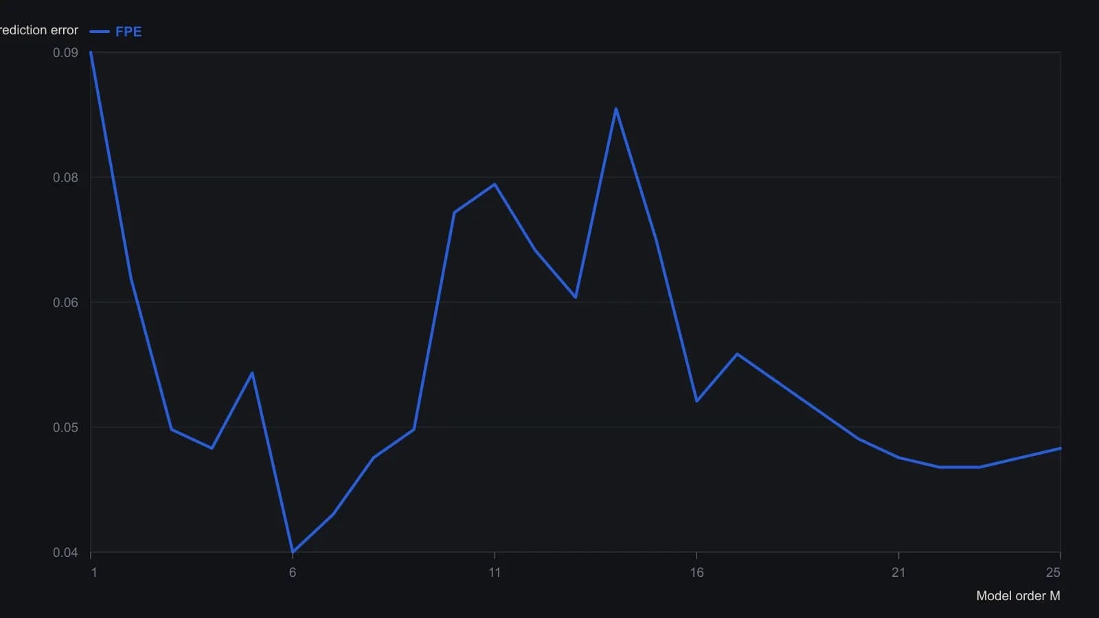
The source computes FPE(M)=(N+M)*P(M)/(N-M) for every order from 1 to 25 and treats a trough as usable only if error does not rise for at least two orders on either side. Digitized from a coarse scan, so FPE readings are approximate to about 0.005.
Which peaks a forecast may inherit
For forecasting, only the lowest-frequency peaks near the dominant cycle are treated as signal. Those peaks are the ones within 15 dB, and the lowest-frequency peak is treated as the prevailing trend. The remaining peaks are treated as interference.
Fourier analysis as a construction check
Fourier analysis is treated as a prerequisite comparison tool because the maximum-entropy spectrum is described as more flexible in adaptation and display, while still being checked against Fourier peak locations on the same series.
Fourier analysis is a classical spectrum estimate used as a construction check on whether maximum-entropy peaks agree in frequency, and more loosely in relative strength, with an independent transform of the same series.
Lowering order and averaging samples
On a 57-week series, final-prediction-error local minima appeared at orders 6 and 16. The order-16 spectrum resolved two significant low-frequency peaks plus noise peaks above 7 cycles per year, and those frequencies generally matched a Fourier spectrum of the same data.
Two-point averaging reduced the series to 28 observations with final-prediction-error minima at orders 2 and 8. The order-8 averaged spectrum kept the dominant-cycle shape with fewer noise peaks and was selected for forecasting while still spanning 16 weeks of lags.
All readings on this track · 28 readings
- 1984Constructing maximum-entropy spectra for dominant-cycle forecasts
- 1984How to construct a maximum-entropy cycle model
- 1984Constructing a maximum-entropy forecast from a chosen lookback
- 1985Constructing period-locked half-cycle and full-cycle averages
- 1986Why Fourier windows limit dominant-cycle resolution
- 1987Assembling short-lookback maximum-entropy cycle forecasts
- 1988Why a fitted dominant cycle is not a forecast
- 1989Evaluating commodity cycle personalities with spectral histograms
- 1989Evaluating next-session cycle forecasts with stops
- 1989Constructing cycle-aged volatility trailing stops
- 1990A channel signal-to-noise gate for dominant-cycle forecasts
- 1990Year-over-year dominant cycle personality audit
- 1991Cyclic entry from a locked dominant-cycle phase
- 1992Stationarity states on synchronized futures spectral contours
- 1997Hidden horizon assumptions in dominant-cycle readings
- 1997When market cycles are absent more than present
- 1997A spectral estimator that retunes indicators to the measured cycle
- 2000Constructing a Hilbert dominant cycle and a maximum-entropy refinement
- 2000Switch trend and cycle indicators after a half-cycle dwell test
- 2000Constructing a dominant-cycle squelch trend filter
- 2000Phasor displays for dominant-cycle construction
- 2002Low-lag trendline from elliptic and dominant-cycle notches
- 2004Spectral peaks are mode diagnostics, not forecasts
- 2004Compressive last-stage oscillator construction
- 2013Constructing trend failure curves from qualified-trend transitions
- 2014Lookback range, a two-lag smoother, and next-bar fills
- 2014Constructing a MESA stochastic with roofing and SuperSmoother filters
- 2016Constructing spectral heatmaps for dominant market cycles