2013issue C1128-33
Constructing a repeated-median slope as a resistant trend filter
A velocity system issues trades only after the slope of a line fitted through N past prices crosses an explicit threshold. Least-squares velocity has a breakdown point of 1/N, so one bad observation can change the reading. A repeated-median slope is assembled from nested pairwise medians and attains a 50% breakdown point.
- A trend filter withholds trades until the slope through N past prices crosses a velocity barrier, so signals stay off while prices meander without a notable trend.
- Least-squares velocity is the slope of the line a + b*t that minimizes the sum of squared residuals, and its breakdown point of 1/N means a single bad observation can change the computed velocity.
- Least-absolute-deviation regression has a breakdown point of 29.8%, while a repeated-median slope attains a 50% breakdown point by taking pairwise slopes, reducing each point to the median of those slopes, then taking the median of the pointwise medians.
- In a 15-point demonstration the repeated-median line stays aligned with the uncontaminated unit slope, but market prices still need further nested-median passes because they are not as regularly spaced as that textbook example.
What a velocity system waits for
A velocity system issues trades only after the slope of a line fitted through N past prices crosses an explicit threshold. That threshold is the velocity barrier. The trend filter uses the barrier as a gate, so that signals are withheld while prices meander without a notable trend.
Why one bad print can change least-squares velocity
Ordinary least-squares slope is obtained by minimizing the sum of squared residuals between N prices and the line a + b*t. That estimator is the least-squares velocity. Its breakdown point is 1/N. The breakdown point is the smallest fraction of corrupted observations that can pull a regression coefficient far from the value implied by the uncontaminated data. Because the fraction is 1/N, a single bad observation can change the computed velocity.
Breakdown points for the median and least-absolute-deviation
The sample median of a set of numbers has a breakdown point of 50%, which is the highest breakdown point available. Once half the observations are corrupted, the good and bad values cannot be distinguished. Least-absolute-deviation regression minimizes the sum of absolute residuals rather than squared residuals. That fit has a breakdown point of 29.8%, so roughly one quarter of the price points can be bad before the fitted intercept and slope become erroneous.
How the repeated-median slope is assembled
A 1982 robust-regression construction for slope attains a 50% breakdown point. For each observation it takes the pairwise slopes through that point, reduces the point to the median of those pairwise slopes, and then takes the median of those pointwise medians. The resulting coefficient is the repeated-median slope.
What a 15-point demonstration shows
In a 15-point demonstration with two contaminated Y values at X positions 10 and 14, the first-stage pairwise slopes from the first point have a median of 1. That reading matches the uncontaminated unit slope. The same demonstration shows the contaminated points pulling the least-squares line toward the outliers, while the repeated-median line remains aligned with the uncontaminated trend.
Further nested-median passes on market prices
Even when the first pairwise-median calculation already recovers the correct slope, further nested-median passes are still required on market prices. Those series are not as regularly spaced as the textbook example.
Fifteen-point demo: outliers pull least-squares off the true slope
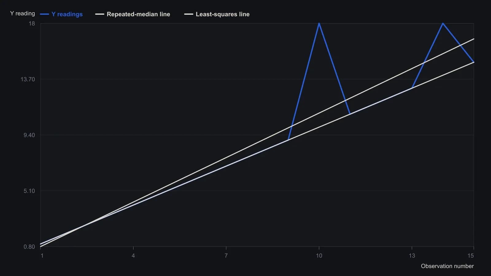
Outliers are Y=18 at X=10 and X=14. The printed least-squares overlay is y=1.1429x−0.3429 (R²=0.8497); the article states the true line as y=x.
Named methods kept in view
The moving average is a smoothing of ordered price, volume, or breadth observations over a defined sampling interval, and it belongs to the same construction family as the slope filters discussed here. The relative-strength index is a bounded oscillator built from ordered price observations over a defined lookback. It is retained here as a named method even though this installment concentrates on slope construction rather than oscillator formulas.
All readings on this track · 33 readings
- 1988Opening-range brackets, a two-bar trend filter, and bounded stops
- 1990Bezier-curve price trend filter
- 1992Constructing a damping-index trend filter
- 1992Building a random walk index trend filter
- 1992Phase diagrams for moving-average trend filters
- 1993Volume-weighted change smoothing and trend ranking
- 1993Concurrent highest-low filter with a largest-low-fall trigger
- 1994Unit-invariant trend filters and the c-test
- 1995Constructing cup and cap entries with a three-bar net line
- 1997Why a daily timing evaluation depends on interval, lookbacks, and the fitting objective
- 2001A volume budget clock for trend-segment construction
- 2001Keep three jobs separate when you test a composite score
- 2002Evaluating the weekly four-percent close filter as a market-state procedure
- 2003Constructing a confirmed zigzag trend filter
- 2004Decompose high, low, and close into separate forecast streams
- 2005Three-state moving-average breakout bar coloring
- 2005Constructing a volume and move-adjusted trend filter
- 2005A fifty-day average breakout as a trend permission filter
- 2005Current-bar inclusion can mute a stochastic channel break
- 2006A stochastic oscillator gated by a long-term exponential average
- 2010A construction test for a modified volume-price trend filter
- 2011Constructing a Spearman rank trend filter
- 2013Constructing a repeated-median slope as a resistant trend filter
- 2014Combining a relative-strength index and trend filters for oversold setups
- 2014Price-rooted lookbacks for a relative strength index, a moving average, and a trend filter
- 2015Evaluating next-session intermarket range forecasts
- 2018Read the intermarket weight matrix first, then the predicted moving-average filter
- 2018Constructing the stiffness trend filter from moving-average holds
- 2018The averaging kernel and the lagged trend gate are separate specifications
- 2019A trend filter is not ready to compare until portfolio constraints are written down
- 2019Lookback, threshold, and position-capacity for a stiffness trend-filter
- 2020Combining a trend filter with a moving average and a stochastic oscillator
- 2020Constructing a relative-strength oscillator with a rank-agreement trend filter