2004issue C051-4
Compressive last-stage oscillator construction
Oscillator building is taught here as a dynamic-range budget. Center and scale a lookback model into the compressive region of an inverse map, then read plus or minus 0.5 as an engineered tripwire rather than as chart decoration.
- Choose a lookback model, recenter and scale it into the compressive region, then apply the inverse map as the last stage.
- The inverse map leaves values inside plus or minus 0.5 nearly unchanged and compresses absolute inputs larger than 2 so the output cannot exceed unit magnitude.
- Mapped polarity is assigned by upward or downward crosses of plus or minus 0.5, with a precedence clause so only one polarity is active.
- Confining the mapped waveform to plus or minus 1 keeps total wave energy finite, which the source ties to guaranteed convergence of some linear-predictive algorithms.
From lookback model to last stage
The historical workflow starts with a lookback model on ordered price observations. That model is recentered and scaled so the working series occupies the compressive region of an inverse map. After the map, reference lines at plus or minus 0.5 are used as decision tripwires.
What the inverse map does
The inverse map leaves inputs inside plus or minus 0.5 nearly unchanged. Absolute inputs larger than 2 are compressed so the output cannot exceed unit magnitude.
The inverse map is described as driving output probability mass toward the poles plus 1 and minus 1. That concentration is why the construction can support two-level decision rules.
Center and scale a relative-strength index
A relative-strength index is a bounded oscillator of consecutive up versus down closes over a stated lookback. Here it is recentered and scaled before the compressive last stage.
A five-bar relative-strength index is recentered by subtracting 50 and scaled by 0.1 so the working series occupies about plus or minus 5 before the inverse map.
That scaled relative-strength series is then smoothed with a nine-bar weighted moving average. The average may be shortened or replaced by an exponential average. The only stated role of the average is to suppress stray crossings.
A saturation wrap versus a reshape
A stochastic oscillator is a range-normalization wrap that locates a series between its own recent high and low and thereby forces a fixed 0-100 box. A stochastic oscillator applied to a relative-strength index is presented as a saturation wrap that forces that box.
The inverse map is offered as a substitute that reshapes the same oscillator's distribution without that wrap.
Tripwires at plus or minus 0.5
The mapped relative-strength series is plotted with reference lines at plus and minus 0.5. Polarity is assigned by upward versus downward crosses of either line. A precedence clause keeps only one polarity active.
Inverse Fisher RSI on QQQ with ±0.5 tripwires
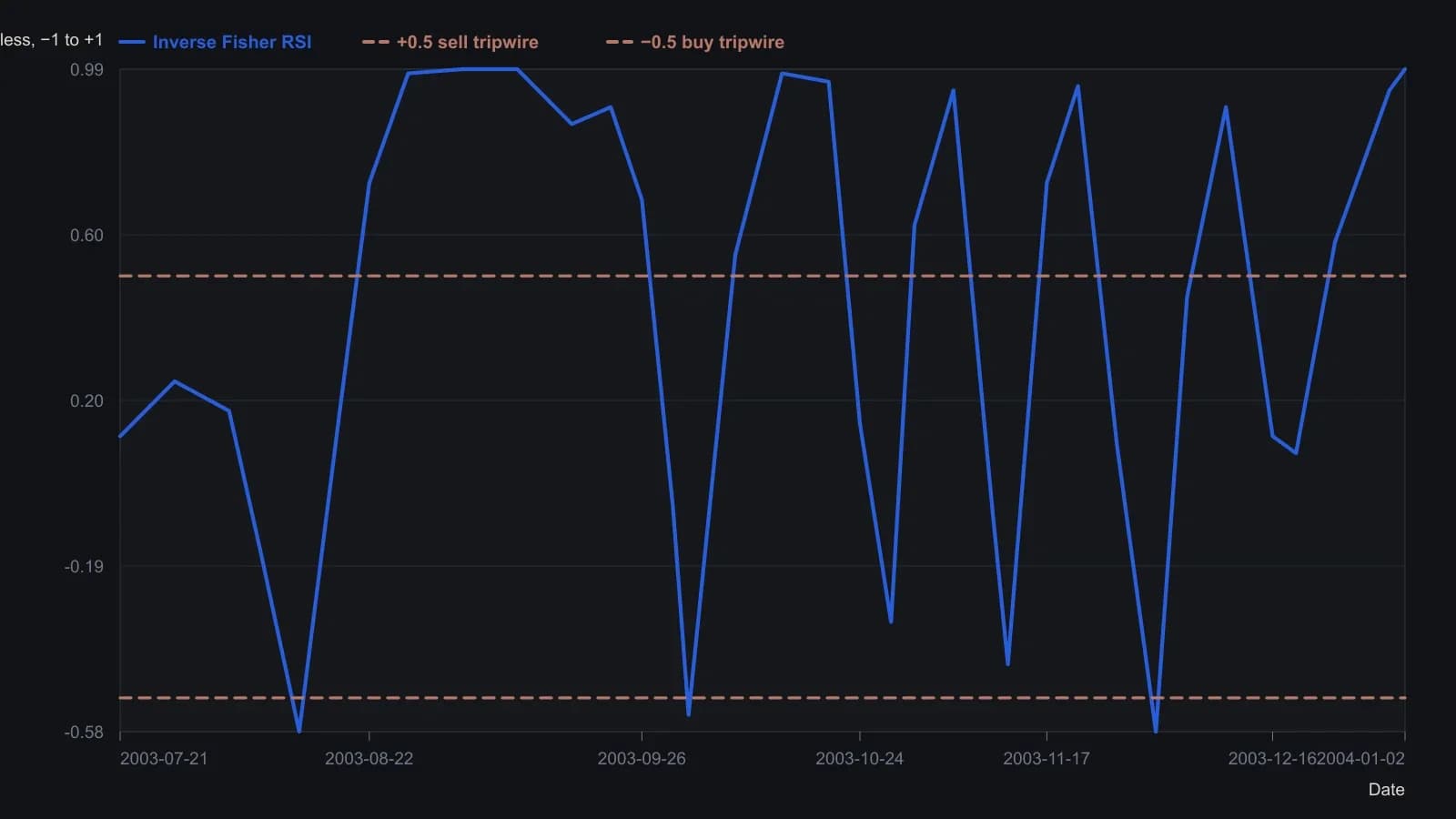
Five-bar RSI translated by 50 and scaled by 0.1, then nine-bar weighted-average smoothed before the inverse Fisher map. Digitized from the raster: turning points placed to the nearest few sessions, amplitudes to about 0.05. Last printed reading on the pane is 0.99.
The same last stage on a cycle residual
A cycle-isolation filter is a short binomial smoother plus a two-pole high-pass recurrence that extracts a variable-amplitude cyclic residual from midpoint price.
The historical filter uses midpoint price, a four-bar binomial smooth, a two-pole recurrence with alpha equal to 0.07, and a second-difference substitute for the first seven bars. That residual then passes through the same inverse map.
The unmapped cycle residual is timed by a cross of the series with its own one-bar lag. The mapped residual uses the same plus or minus 0.5 reference lines as the relative-strength construction.
Finite energy and a linear-predictive spectrum
Because the mapped waveform is confined to plus or minus 1, total wave energy is finite. The source states that some linear-predictive algorithms are then guaranteed to converge.
Maximum-entropy spectrum analysis is a linear-predictive spectral estimator. It is named as a spectral method already applied to traded series, in the same closing discussion that links finite wave energy to linear-predictive convergence.
All readings on this track · 28 readings
- 1984Constructing maximum-entropy spectra for dominant-cycle forecasts
- 1984How to construct a maximum-entropy cycle model
- 1984Constructing a maximum-entropy forecast from a chosen lookback
- 1985Constructing period-locked half-cycle and full-cycle averages
- 1986Why Fourier windows limit dominant-cycle resolution
- 1987Assembling short-lookback maximum-entropy cycle forecasts
- 1988Why a fitted dominant cycle is not a forecast
- 1989Evaluating commodity cycle personalities with spectral histograms
- 1989Evaluating next-session cycle forecasts with stops
- 1989Constructing cycle-aged volatility trailing stops
- 1990A channel signal-to-noise gate for dominant-cycle forecasts
- 1990Year-over-year dominant cycle personality audit
- 1991Cyclic entry from a locked dominant-cycle phase
- 1992Stationarity states on synchronized futures spectral contours
- 1997Hidden horizon assumptions in dominant-cycle readings
- 1997When market cycles are absent more than present
- 1997A spectral estimator that retunes indicators to the measured cycle
- 2000Constructing a Hilbert dominant cycle and a maximum-entropy refinement
- 2000Switch trend and cycle indicators after a half-cycle dwell test
- 2000Constructing a dominant-cycle squelch trend filter
- 2000Phasor displays for dominant-cycle construction
- 2002Low-lag trendline from elliptic and dominant-cycle notches
- 2004Spectral peaks are mode diagnostics, not forecasts
- 2004Compressive last-stage oscillator construction
- 2013Constructing trend failure curves from qualified-trend transitions
- 2014Lookback range, a two-lag smoother, and next-bar fills
- 2014Constructing a MESA stochastic with roofing and SuperSmoother filters
- 2016Constructing spectral heatmaps for dominant market cycles