2000issue C031-7
Constructing a Hilbert dominant cycle and a maximum-entropy refinement
This archive article reconstructs a dominant-cycle reading as a sequence of design choices: set observation-window-lag, form a zero-lag-average, split the detrended series with a Hilbert-transform, gate the phasor by signal-to-noise-ratio, then let the instantaneous frequency set the history length of a maximum-entropy-spectrum estimate.
- A uniformly weighted average plotted at the right edge lags by half the window width, and a linearly weighted average lags by one-third of that width, so observation-window-lag is an explicit design knob.
- After detrending, a Hilbert-transform builds in-phase and quadrature traces so a phasor can report amplitude and bar-to-bar phase for spectral-analysis.
- Dominant-cycle period is the bar count recovered by accumulating phase change to a full rotation; that instantaneous frequency then sets how much history a maximum-entropy-spectrum estimate may use.
- Cycle readings are treated as usable only when the signal-to-noise-ratio exceeds 6 dB, and a lengthening instantaneous period is read as departure from a cyclic turning point into a trend.
A constructed cycle reading
The historical workflow treats a dominant-cycle reading as a chain of constructed instruments rather than as a property read off the chart. Lag is chosen first. The series is then detrended, split into orthogonal components, gated by a signal-to-noise-ratio test, and only then passed to a maximum-entropy-spectrum estimate whose history length is set by the instantaneous frequency.
Lag as a design knob
A uniformly weighted average plotted at the right edge of its observation window produces observation-window-lag of half the window width. A linearly weighted average lags by one-third of that width.
On a constant-slope input the exponential-smoothing-constant equals 1 divided by lag plus 1, so a three-bar lag uses 0.25. A related mapping of 2 divided by period plus 1 follows because a simple average lags by about half its period. The constant is therefore fixed once a tolerable lag is chosen.
Reconstructing a linear trend without lateral delay
A zero-lag-average on a linear trend is a causal reconstruction. It adds the vertical gap between a lag-L average and a lag-2L average back onto the first average so the linear trend is recovered without lateral delay.
Choosing a four-bar lag hides cycle periods shorter than about four bars. A two-pass forward-then-backward average cancels lag only if future bars are available at the right edge.
In-phase and quadrature after the detrend
Spectral-analysis here means decomposing a detrended price series into frequency, amplitude, and phase by forming orthogonal in-phase and quadrature components. After the detrend, a Hilbert-transform all-pass construction synthesizes those traces from a single real sampled series so phase and amplitude can be read bar by bar.
The implemented transform carries about four bars of lag, which is a half-cycle on an eight-bar oscillation and can invert the apparent turning-point crossings. That lag is part of the instrument, not a later correction.
A decibel gate on the phasor
A phasor is applied only after the series is detrended. Signal amplitude is the phasor length formed from the squared in-phase and quadrature terms. Noise is defined as a smoothed bar range.
The signal-to-noise-ratio is reported in decibels: 0 dB when signal equals noise, and 6 dB when signal amplitude is twice the noise amplitude. The ratio is the test of whether a cycle reading is distinguishable from sampling uncertainty.
Accumulating phase into a period
Instantaneous cycle period is formed by taking the arctangent of quadrature over in-phase, differencing that phase from bar to bar, and summing the increments backward until they reach 360 degrees. A 10-bar cycle corresponds to 36 degrees of phase per bar.
The dominant-cycle is that prevailing oscillatory period after the bar count is smoothed into a usable cycle length. The Hilbert instantaneous frequency is presented as finer than a fast Fourier measurement.
Setting the spectral history length
A maximum-entropy-spectrum is then used to shrink the effective noise bandwidth. The instantaneous frequency measurement sets how much history is fed into that cycle estimate, so the data length of the spectral reading is not an independent free parameter.
When the period lengthens
On the assembled indicators, cycle readings are treated as usable only when the signal-to-noise-ratio exceeds 6 dB. A lengthening instantaneous period, illustrated peaking at 34 after a major low, is interpreted as departure from a cyclic turning point into a trend.
Hilbert dominant-cycle period on daily S&P
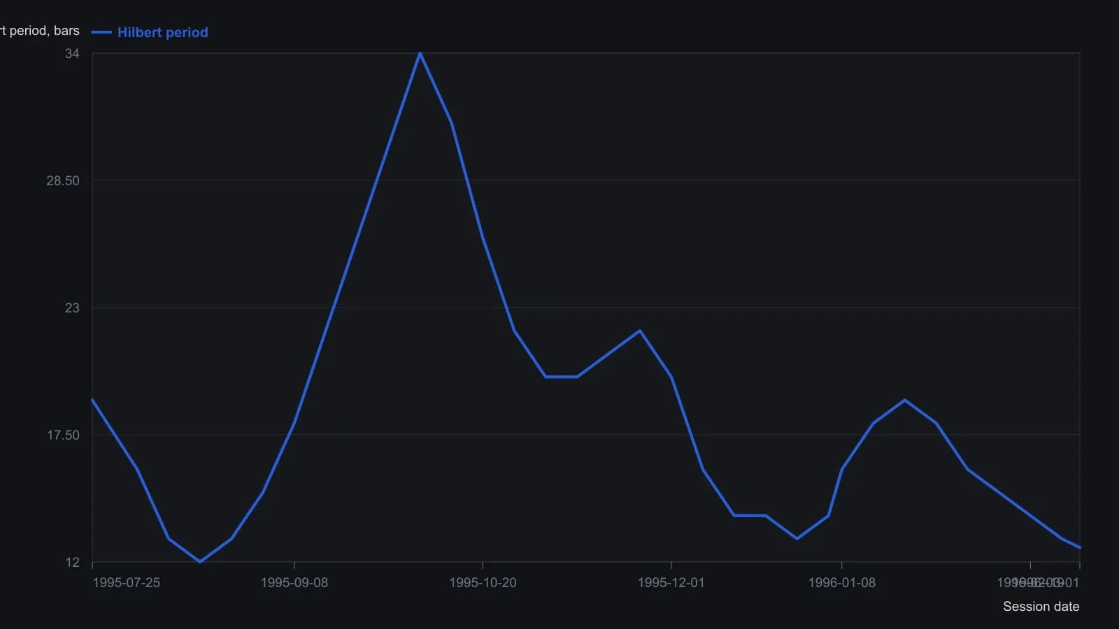
Pane is the Hilbert instantaneous period after the article's 0.25/0.75 EMA smooth. The 34-bar peak and the 16-bar January reading are stated in the article; other points are approximate raster readings rounded to the nearest bar.
All readings on this track · 28 readings
- 1984Constructing maximum-entropy spectra for dominant-cycle forecasts
- 1984How to construct a maximum-entropy cycle model
- 1984Constructing a maximum-entropy forecast from a chosen lookback
- 1985Constructing period-locked half-cycle and full-cycle averages
- 1986Why Fourier windows limit dominant-cycle resolution
- 1987Assembling short-lookback maximum-entropy cycle forecasts
- 1988Why a fitted dominant cycle is not a forecast
- 1989Evaluating commodity cycle personalities with spectral histograms
- 1989Evaluating next-session cycle forecasts with stops
- 1989Constructing cycle-aged volatility trailing stops
- 1990A channel signal-to-noise gate for dominant-cycle forecasts
- 1990Year-over-year dominant cycle personality audit
- 1991Cyclic entry from a locked dominant-cycle phase
- 1992Stationarity states on synchronized futures spectral contours
- 1997Hidden horizon assumptions in dominant-cycle readings
- 1997When market cycles are absent more than present
- 1997A spectral estimator that retunes indicators to the measured cycle
- 2000Constructing a Hilbert dominant cycle and a maximum-entropy refinement
- 2000Switch trend and cycle indicators after a half-cycle dwell test
- 2000Constructing a dominant-cycle squelch trend filter
- 2000Phasor displays for dominant-cycle construction
- 2002Low-lag trendline from elliptic and dominant-cycle notches
- 2004Spectral peaks are mode diagnostics, not forecasts
- 2004Compressive last-stage oscillator construction
- 2013Constructing trend failure curves from qualified-trend transitions
- 2014Lookback range, a two-lag smoother, and next-bar fills
- 2014Constructing a MESA stochastic with roofing and SuperSmoother filters
- 2016Constructing spectral heatmaps for dominant market cycles