2013issue C0740-43
Constructing trend failure curves from qualified-trend transitions
A qualified-trend can carry a mean-time-to-failure curve so duration after the transition is treated as an estimable life-cycle quantity. Confirmed-trend and suspect-trend volume tags, window length, and group membership are separate construction axes, and the curve is specified as a support measure beside other qualification techniques.
- Attach a mean-time-to-failure curve after a qualified-trend transition so remaining duration is an estimable life-cycle quantity rather than an unmeasured remainder.
- Treat confirmed-trend and suspect-trend volume tags as a second construction axis, because those labels were observed to carry different continuance associations.
- Give the same instrument failure curves on more than one time frame so time-frame-alignment can show whether duration risk is clustered or mixed.
- Keep the duration curve as a support-not-primary measure beside other qualification techniques.
Treat duration as a construction step
A qualified-trend is a directional regime labeled after a systematic transition and further tagged as confirmed or suspect by whether volume agrees at the turn. Once that label exists, a mean-time-to-failure style curve can be attached so duration after the transition is treated as an estimable life-cycle quantity rather than an unmeasured remainder.
A mean-time-to-failure reading is an engineering-style estimate of how long a qualified-trend typically lasts before it ends, drawn from a sample of past transitions on a chosen bar count. TradersWeek editorial aim: make that remaining life a measurable construction step rather than a vague cycle guess.
Tag the transition before you estimate life
Build the curve only after the transition is already a qualified-trend. The first construction choice is the volume tag at the turn.
A confirmed-trend is a newly assigned trend whose volume at the transition supports the new direction. A suspect-trend is a newly assigned trend whose volume at the transition fails to confirm the new direction. Those two labels were observed to carry different continuance associations, so each tag is its own construction axis and should not be pooled into one survival path.
Fix the window and the sample
One published construction used about 60 bars per chart, so a daily short-term-window spanned roughly three months of data. That bar count is the sampling interval for the short-term curve. Other windows need their own bar counts and should not be mixed into the same path.
The short-term bullish failure example was built from liquid NYSE, NASDAQ, and AMEX stocks over 2001-11. Exchange-traded notes, exchange-traded funds, and mutual funds were omitted. State the exchange set, the omitted vehicles, and the bar count before you accumulate failures.
Read a rising cumulative-failure-rate
From like-tagged transitions, accumulate the share of trends that have already ended after a given number of bars. That rising share is the cumulative-failure-rate, and it is how acute failure risk is read on the finished curve.
On the constructed short-term curve, the cumulative share of failed trends rose as bar count increased. The speed of that rise depended on both time frame and qualification type. A later bar is therefore a more acute reading only relative to its own window and its own confirmed-trend or suspect-trend tag.
Cumulative failure rates for short-term bullish trends
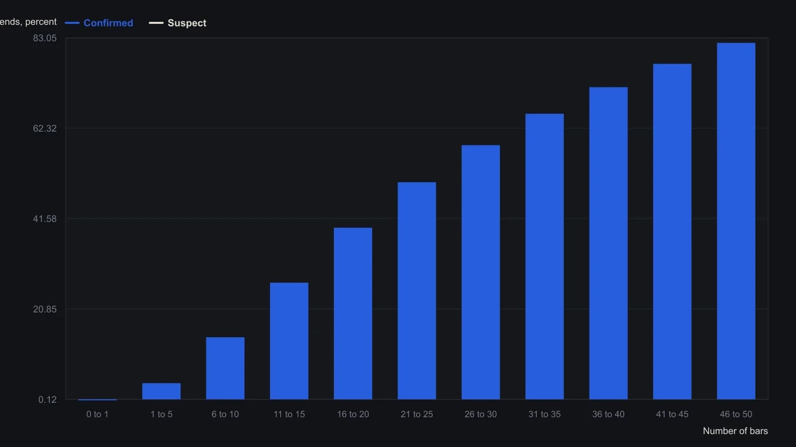
The source study used approximately 60-bar charts of liquid NYSE, NASDAQ, and AMEX stocks over 2001–11, excluding ETNs, ETFs, and mutual funds. The figure header on the same panel calls the case a bullish-to-sideways transition on the intermediate-term frame and dates the sample 2002–11.
Compare windows on the same instrument
The same instrument can be given failure curves on more than one time frame so clustered high or low readings become an explicit time-frame-alignment check rather than a single-horizon view.
Time-frame-alignment compares high versus low failure readings on the same instrument across short, intermediate, and long windows. Clustered high or low readings are a shared duration picture. Mixed high and low readings are a mixed picture.
Estimate a group-level-curve separately
A further construction path is to estimate failure curves for sector or industry groups separately. A group-level-curve is a failure-rate construction for a sector or industry cohort rather than the full liquid-stock population.
Those group populations were described as unlike the all-stock curve. Do not assume a sector or industry life cycle matches the market-wide liquid-stock path.
Read a historical long-horizon snapshot
In a July 2012 long-horizon S&P 500 example, a confirmed bullish trend at a 20-bar age was assigned a 60 percent mean-time-to-failure reading, with the next month described as just over 72 percent. That pair is a historical construction snapshot on one instrument, one confirmed-trend tag, and one horizon. It is not a template for other tags, windows, or dates.
Keep the curve beside other qualification tools
The finished object is a support-not-primary measure: a duration curve that sits beside other qualification tools and is not treated as the sole decision engine. Construction stops at an estimable life-cycle reading for an already-tagged trend. It does not replace the transition rules that created the qualified-trend.
Editorial reading of cycle baselines
A maximum-entropy-spectrum construction estimates the frequency content of an ordered price, volume, or breadth series from a defined lookback so a cycle baseline can be compared with a later out-of-sample window. A dominant-cycle is the strongest repeating interval isolated from ordered market observations over a stated sampling interval and lookback, used as an explicit cycle baseline rather than a visual guess. Spectral-analysis is the broader construction of frequency structure from ordered observations so cycle length and persistence can be measured against a defined sampling interval.
TradersWeek editorial reading: those spectral constructions supply an explicit cycle baseline. The mean-time-to-failure curve supplies an explicit duration construction after a qualified-trend transition. The archive facts describe the failure-curve workflow only. The editorial point is to keep both as measured construction steps rather than substituting a vague cycle guess for either.
All readings on this track · 28 readings
- 1984Constructing maximum-entropy spectra for dominant-cycle forecasts
- 1984How to construct a maximum-entropy cycle model
- 1984Constructing a maximum-entropy forecast from a chosen lookback
- 1985Constructing period-locked half-cycle and full-cycle averages
- 1986Why Fourier windows limit dominant-cycle resolution
- 1987Assembling short-lookback maximum-entropy cycle forecasts
- 1988Why a fitted dominant cycle is not a forecast
- 1989Evaluating commodity cycle personalities with spectral histograms
- 1989Evaluating next-session cycle forecasts with stops
- 1989Constructing cycle-aged volatility trailing stops
- 1990A channel signal-to-noise gate for dominant-cycle forecasts
- 1990Year-over-year dominant cycle personality audit
- 1991Cyclic entry from a locked dominant-cycle phase
- 1992Stationarity states on synchronized futures spectral contours
- 1997Hidden horizon assumptions in dominant-cycle readings
- 1997When market cycles are absent more than present
- 1997A spectral estimator that retunes indicators to the measured cycle
- 2000Constructing a Hilbert dominant cycle and a maximum-entropy refinement
- 2000Switch trend and cycle indicators after a half-cycle dwell test
- 2000Constructing a dominant-cycle squelch trend filter
- 2000Phasor displays for dominant-cycle construction
- 2002Low-lag trendline from elliptic and dominant-cycle notches
- 2004Spectral peaks are mode diagnostics, not forecasts
- 2004Compressive last-stage oscillator construction
- 2013Constructing trend failure curves from qualified-trend transitions
- 2014Lookback range, a two-lag smoother, and next-bar fills
- 2014Constructing a MESA stochastic with roofing and SuperSmoother filters
- 2016Constructing spectral heatmaps for dominant market cycles