2012issue C0740-44
A 2012 case study in Kondratieff-wave and presidential-cycle overlays
A 2012 overlay joined a Kondratieff-wave path, a presidential-cycle template, and chart-based cycle counts. TradersWeek reads that stack, as editorial commentary, as a case in placing one year inside overlapping regimes rather than treating any single calendar as a forecast.
- The Kondratieff-wave was framed as a 54- to 55-year economic boom-and-bust cycle whose bust phase was a renunciation of debt, not a direct stock-market clock.
- Anticipation-lag on a monthly S&P 500 overlay put index lows at least two years ahead of economic-wave turns and let tops run a year or two past those turns.
- Each dominant-cycle count had to stay a subdivision of the 54-year wave, so a six-year gap between the 2003 and 2009 lows was rejected as a buy-and-hold span.
- The presidential-cycle was party-independent: reelection years were associated with a continued S&P rise, and a new president with possible weakness in the first year to year and a half.
A risk-off backdrop and a stacked calendar
The archive framed 2011 as a risk-off year. Cash preference, eurozone stress centered on Greece and Italy, and the March 11 Japan disaster were treated as the prevailing market backdrop. From that setting the source laid a long economic wave, a four-year political calendar, and chart-based cycle counts over the same price history.
The long wave as economic context
The Kondratieff-wave was stated as a 54- to 55-year economic boom-and-bust cycle. Its bust phase was characterized as a renunciation of debt, not as a direct stock-market clock. The author treated the long wave as an economic forecast and argued that index bottoms should print earlier than the wave and index tops later, because markets anticipate the economy.
A projected wave chart extended labeled panic, good-time, and hard-time intervals out to 2039. The 54-year span was required to subdivide into 27-year groups such as 10+8+9 and 11+9+7. Those shorter counted intervals are the dominant-cycle layer in this case.
Anticipation-lag on the monthly overlay
On a monthly S&P 500 overlay, index lows were described as leading economic-wave turns by at least two years, while tops ran a year or two past those turns. That lead and lag is the anticipation-lag used here. The same overlay kept the long wave in a bullish regime after 2012, with a first major correction placed in 2016 and a continued rise discussed into 2019 to 2020, after earlier panic markers near 1999 and 2007.
Dominant-cycle counts stay inside the wave
A six-year gap between the 2003 and 2009 lows was noted as historically tempting to treat as a buy-and-hold span. The archive rejected that reading because each counted dominant-cycle had to remain a subdivision of the 54-year wave.
A party-independent presidential cycle
The presidential-cycle was presented as a four-year seasonal template that does not depend on which party holds office. Reelection years were associated with a continued S&P rise. A new president was associated with possible weakness in the first year to year and a half.
Combining the still-rising long-wave path into 2016 with that election-year pattern, the source treated 2012 as consistent with an incumbent remaining in office and a change of party only later, around 2017.
Chart structure as the joining layer
An elliott-wave count of impulse and corrective swings supplied that technical structure. It turned the same price history into a falsifiable path hypothesis. Seasonal analysis supplied the regime stack. Dominant-cycle detection supplied the explicit subdivisions of the long wave.
Quarterly S&P 500, 1970–2011
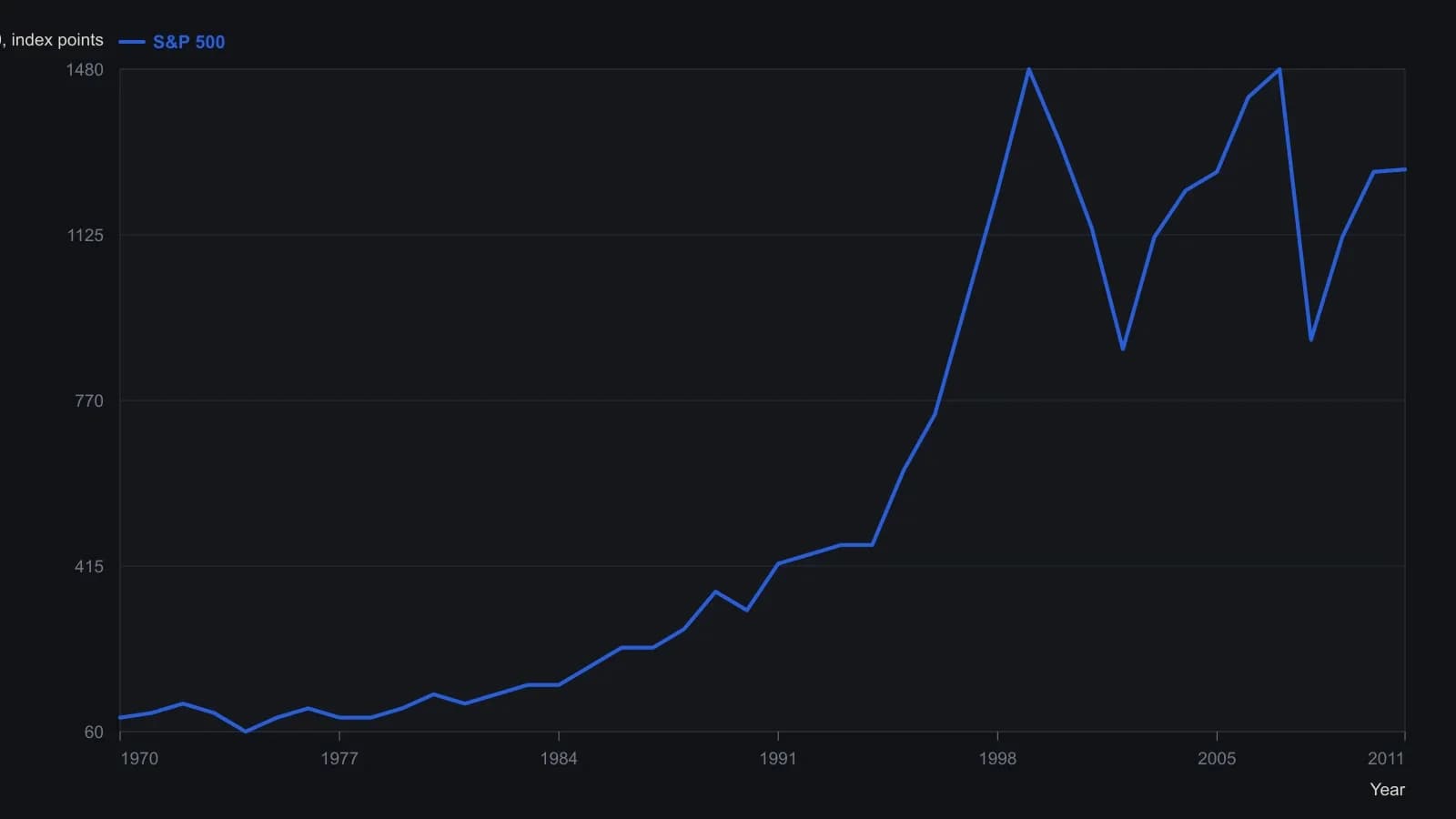
Year-end readings, rounded to 20 index points, because the pane plots four decades on a linear scale to 2,000 and the 1970s candles sit on the bottom of the frame. Pattern letters A–F and the September 2012 projection are not redrawn.
How one year sits inside the stack
Editorial note: TradersWeek reads the 2012 stack as a case in placing a single year inside concurrent calendars instead of treating any single calendar as a forecast. That sentence is editorial. The archive joined the still-rising long-wave path to the election-year pattern and asked for technical structure before using the election overlay.
All readings on this track · 21 readings
- 1986Two gates for setup and operator readiness
- 1990Time-only cycle dates in a Treasury bond case study
- 1990Constant-dollar regimes, the value line, and nested cycles
- 1992The four-year election cycle as an equity regime map
- 1992A semiconductor seasonal-index before the relative-strength overlay
- 1992Lock the holiday window as a regime, then veto resistance
- 1995Regime-aware stock screening with intermarket context
- 1996Standard-error bands, width gates, and weekday counts
- 1999Constructing seasonal factors from centered moving averages
- 2000Seasonal window, then weekly breadth
- 2004Copper as a regime map for cycles and recessions
- 2008Election-cycle windows as a mechanical seasonal system
- 2012A 2012 case study in Kondratieff-wave and presidential-cycle overlays
- 2012The October to May window as a mechanical portfolio procedure
- 2013Half-year seasonality as an equity regime overlay
- 2014Seasonal cycles as a regime overlay
- 2015Seasonal oil window as a defined-risk spread case
- 2017Calendar regimes, RSI events, and sector rotation rules
- 2018Seasonal windows as testable entry and abstention rules
- 2019Calendar rotation of seasonal and regime questions
- 2020Constructing calendar interval votes for cycle workbooks