2013issue C0522-25
Half-year seasonality as an equity regime overlay
From 1979 to 2012, S&P 500 calendar halves differ in index points and still differ in percentage return, worst-case depth, and half-year Sharpe. The historical workflow treats that average, exceptions included, as a seasonal overlay for long aggressiveness and stop tightness.
- The historical workflow treats the November-April and May-October windows as a seasonal overlay that raises or lowers long aggressiveness and stop tightness, not as a stand-alone calendar system.
- Point-change bias overweights later years in raw index-point totals, which is why the split is also compared on percentage changes.
- On a percentage basis the November-April window still showed a higher best reading, a milder worst reading, and a better half-year Sharpe, while leading in 22 of 33 years.
- Editorial view: a seasonal pattern with frequent exceptions can still serve as regime context for a single equity idea without becoming a complete system.
What the long sample records
The archive follows the S&P 500 from November 1979 through November 2012, a span in which the index moved from 101.82 to 1,412.16. The case is built around two complementary six-month regimes: the November-April window, conventionally ending in April and treated as the historically stronger equity half-year, and the May-October window treated as the weaker seasonal regime.
Over that span, net index-point change was +1,380.8 across November-April halves and -70.4 across May-October halves.
Why point totals misstate the split
Nominal point totals overweight later years because each percentage move equals more points at higher index levels. That point-change bias is why the comparison is also run on percentage changes.
Percentage windows still differ
Average half-year change was 7.3 percent (15.1 percent annualized) in the November-April window versus 1.9 percent (3.9 percent annualized) in the May-October window, a 5.4 percentage-point average gap.
In the tabulated sample, the November-April half had a higher best reading (24.1 percent versus 19.9 percent) and a milder worst reading (-12.6 percent versus -30.1 percent) than the May-October half. Half-year standard deviation was 9.9 percent versus 10.7 percent. Half-year Sharpe ratios were 0.23 versus -0.29 when a 5 percent risk-free rate is assumed.
Exceptions inside the average
In 22 of the 33 years examined, the November-April half outperformed the May-October half.
The 2008 May-October half fell 30.1 percent, compared with a 10.6 percent decline in the November-April span counted as ending in April 2008. The six months ended April 1987 gained 18.2 percent and preceded that year's October break.
A later subsample
In the November 1994 through November 2012 subsample, average half-year changes were 6.8 percent versus 0.7 percent. The November-April window led in 13 of 18 years, and half-year Sharpe ratios using a 2 percent risk-free rate were 0.48 versus -0.11.
Used as a seasonal overlay
The split is treated as an average with frequent exceptions and is used to raise or lower long aggressiveness and stop tightness rather than as a stand-alone calendar system.
Editorial reading: the calendar half is context for how a single equity idea is sized and risk-managed, not a buy-or-sit-out rule.
S&P 500 half-year percentage returns, 1980–2012
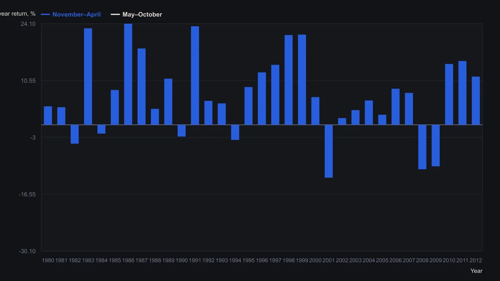
Figure 1 lists October 1979 as a starting index level only; percentage half-year returns begin with the 1980 row. 2008’s May–October drop of −30.1% is the sample’s worst printed half.
All readings on this track · 21 readings
- 1986Two gates for setup and operator readiness
- 1990Time-only cycle dates in a Treasury bond case study
- 1990Constant-dollar regimes, the value line, and nested cycles
- 1992The four-year election cycle as an equity regime map
- 1992A semiconductor seasonal-index before the relative-strength overlay
- 1992Lock the holiday window as a regime, then veto resistance
- 1995Regime-aware stock screening with intermarket context
- 1996Standard-error bands, width gates, and weekday counts
- 1999Constructing seasonal factors from centered moving averages
- 2000Seasonal window, then weekly breadth
- 2004Copper as a regime map for cycles and recessions
- 2008Election-cycle windows as a mechanical seasonal system
- 2012A 2012 case study in Kondratieff-wave and presidential-cycle overlays
- 2012The October to May window as a mechanical portfolio procedure
- 2013Half-year seasonality as an equity regime overlay
- 2014Seasonal cycles as a regime overlay
- 2015Seasonal oil window as a defined-risk spread case
- 2017Calendar regimes, RSI events, and sector rotation rules
- 2018Seasonal windows as testable entry and abstention rules
- 2019Calendar rotation of seasonal and regime questions
- 2020Constructing calendar interval votes for cycle workbooks