2018issue C0418-21
Pair two adaptive averages to filter swing turns
An adaptive moving average that rescales from where the close sits in the lookback high-low range can be read beside a Kaufman adaptive moving average that rescales from an efficiency ratio. Editorial reading: treat their joint turning points as a swing-trading filter so an entry is a test of agreement, not a single lagging line.
- The adaptive moving average updates from a multiplier that locates the close inside the lookback high-low range rather than from Kaufman's efficiency ratio.
- The multiplier stays between zero and one, sits near 0.8 to 1 when price is near the period high or low, and equals zero when the close is mid-range.
- The two averages can be paired so one tracks price more closely while their joint turning points filter later movement, preferably when the price swing is relatively large.
- Because both averages are lagging-style indicators, the crossover system can issue relatively late signals and was suggested with price analysis and a relative-strength index.
Range location versus path efficiency
The adaptive moving average updates from a multiplier that locates the current close inside the lookback high-low range rather than from Kaufman's efficiency ratio. The Kaufman adaptive moving average instead rescales its smoothing from an efficiency ratio of net close-to-close change over the lookback to the sum of one-period close changes.
A moving average remains the smoothed baseline path against which these adaptive variants are compared. The two adaptive series change how quickly that path updates, but they do not use the same location rule.
How the multiplier is built
Typical adaptive-average settings use a 10-period lookback with fastest and slowest exponential constants of 2 and 30 periods, and those constants can be changed to match holding style.
The multiplier equals the absolute difference between close-to-low and high-to-close distances divided by the lookback high-low span, using a 10-plus-1 range window. The multiplier stays between zero and one, sits near 0.8 to 1 when price is near the period high or low, and equals zero when the close is mid-range.
Shared smoothing and a parallel table
The adaptive smoothing constant squares a blend of the multiplier with the fastest and slowest exponential constants, following the same squared-constant construction used for the Kaufman average.
A worked price table computes both averages in parallel from the same highs, lows, and closes, showing distinct multiplier, efficiency-ratio, and smoothing-constant columns for each.
Crossovers as a swing-trading filter
The two averages can be paired so that one tracks price more closely while their joint turning points are used to filter subsequent price movement.
A swing-trading procedure that marks bullish and bearish crossovers of the two averages produced mixed signals on a Dow Jones Industrial Average chart and was described as working better when price swings were relatively large, specifically when prices were up over 5 percent.
Late signals and companion checks
Because both averages are lagging-style indicators, the crossover system can issue relatively late signals and was suggested for use with price analysis and a relative-strength index to mark overbought and oversold zones.
DJIA with AMA and KAMA as a swing-turn filter
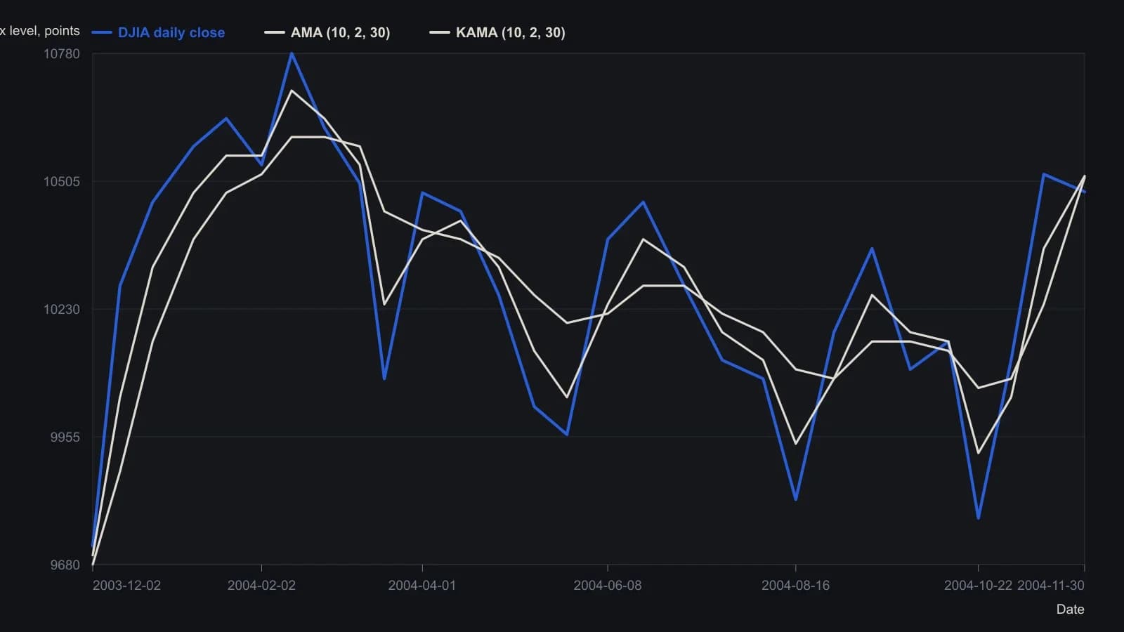
Both averages use the article’s default 10/2/30 settings. Apirine notes the pair behaves better when the swing is larger than about 5 percent and that two lagging lines can still fire late. Intra-month dates are inferred from the monthly axis labels; interior levels are raster estimates to about 20 index points.
All readings on this track · 24 readings
- 1991Building variable-length moving averages from partitioned price changes
- 1991Variable-length moving average from change dispersion
- 1992Constructing volatility-adaptive exponential smoothing
- 1995Constructing an adaptive moving average with an efficiency ratio and filter
- 1995Two-gate breakout confirmation with adaptive averages
- 1995Building momentum-scaled adaptive moving averages
- 1995Adaptive length as a construction choice inside exponential smoothing
- 1998Testing price-channel breakouts with a lag-aware adaptive average
- 1998Constructing filters by nesting offsets and variable weights
- 1998Constructing an efficiency ratio adaptive average and entry filter
- 2001Encoding candle structure as a numeric filter
- 2001Adaptive averages driven by cycle-phase speed
- 2005Constructing an adaptive moving average from a fractal-dimension weight
- 2005Range-dimension adaptive exponential filter
- 2010Constructing simple, exponential, and adaptive averages
- 2010How a price-hugging smoother is assembled from ordinary averages
- 2013Evaluating an adaptive moving average against a same-window moving average
- 2016Three-layer confirmation: adaptive average, stochastic relative strength index, and stop-and-reverse
- 2017One-alpha reverse-path exponential smoothing
- 2018Pair two adaptive averages to filter swing turns
- 2018Two Adaptive moving averages as a confirmation pair
- 2018Constructing an adaptive filter for adoption-cycle reversals
- 2018Constructing a deviation-scaled adaptive moving average
- 2020Walk-forward and adaptive averages as two tests of the same trend