2018issue C078-11
Constructing a deviation-scaled adaptive moving average
A deviation-scaled moving average first locks exponential alpha to a critical period, then multiplies that baseline by the absolute amplitude of a whitened two-bar residual expressed in its own root-mean-square units.
- An exponential moving average mixes the current close with the previous filter value through an alpha that lies between zero and one.
- Common adaptive modifiers estimated over several bars add computational lag before they can change that alpha.
- A deviation-scaled-moving-average multiplies a critical-period baseline alpha by the absolute amplitude of a whitened two-bar residual expressed in rms-scale units.
- A single user period sets both the baseline alpha and the root-mean-square window that measures local scale.
Two stages of construction
A deviation-scaled-moving-average is assembled in two stages. First, an exponential baseline is locked to a user-chosen critical-period. Second, a whitened two-bar residual, expressed in its own rms-scale units, raises or lowers the mixing weight from that baseline.
An exponential mix and its alpha
An exponential moving average is built as a convex mix of the current close and the previous filter value. The mixing weight is alpha, which lies between zero and one. Smaller alpha increases smoothing. Larger alpha reduces smoothing and gives more weight to the latest close.
Why common adaptive modifiers add lag
Adaptive averages change that alpha from a separately measured market condition. Two common constructions derive the modifier from an RSI-like statistic or from net price change over a window divided by the sum of bar-to-bar changes. Both estimate the modifier over multiple bars, which adds computational lag.
A critical-period baseline
The user period is treated as the filter critical-period, the cycle length at which passed signal power is halved. The baseline exponential alpha is set to five divided by that period. When the oscillator’s scaled amplitude deviation equals one, the adaptive alpha matches an exponential average with the same critical-period.
A zeros-oscillator and spectrum-whitening
The scaling oscillator is a two-bar close-to-close difference. This zeros-oscillator has a transfer response of zero for an unchanging series, which supplies a nominal zero mean, and it rolls off at six decibels per octave. Fractal market amplitudes are described as rising at the same rate, so the difference is used for spectrum-whitening.
The same two-bar difference also has a transfer-response zero at the Nyquist period, the shortest cycle that sampled data can represent. That zero is intended to cancel the six-decibel noise gain of a one-bar difference and to lessen aliasing in the oscillator.
A two-pole residual and rms-scale
The oscillator is passed through a two-pole smoother whose critical-period is half the user period so the residual stays responsive. The smoother coefficients are computed only on the first bar. Because the input is nominally zero-mean, the filtered series is treated as zero-mean as well.
Local scale is the rms-scale of that filtered oscillator over the user period, the root-mean-square of the residual. Dividing the filtered series by that rms-scale expresses it in standard-deviation units. Small local deviation then yields a small effective alpha and heavier smoothing. Large deviation raises alpha and lets the filter follow price more quickly.
Working alpha and the adaptive series
The working alpha is the absolute scaled value times five divided by the period. The adaptive series is the usual exponential recursion that mixes the current close with the previous adaptive value using that working alpha. Tracking speed is retuned by changing the single period input that sets both the baseline alpha and the rms-scale window.
SPY daily with 40-period DSMA, 2017
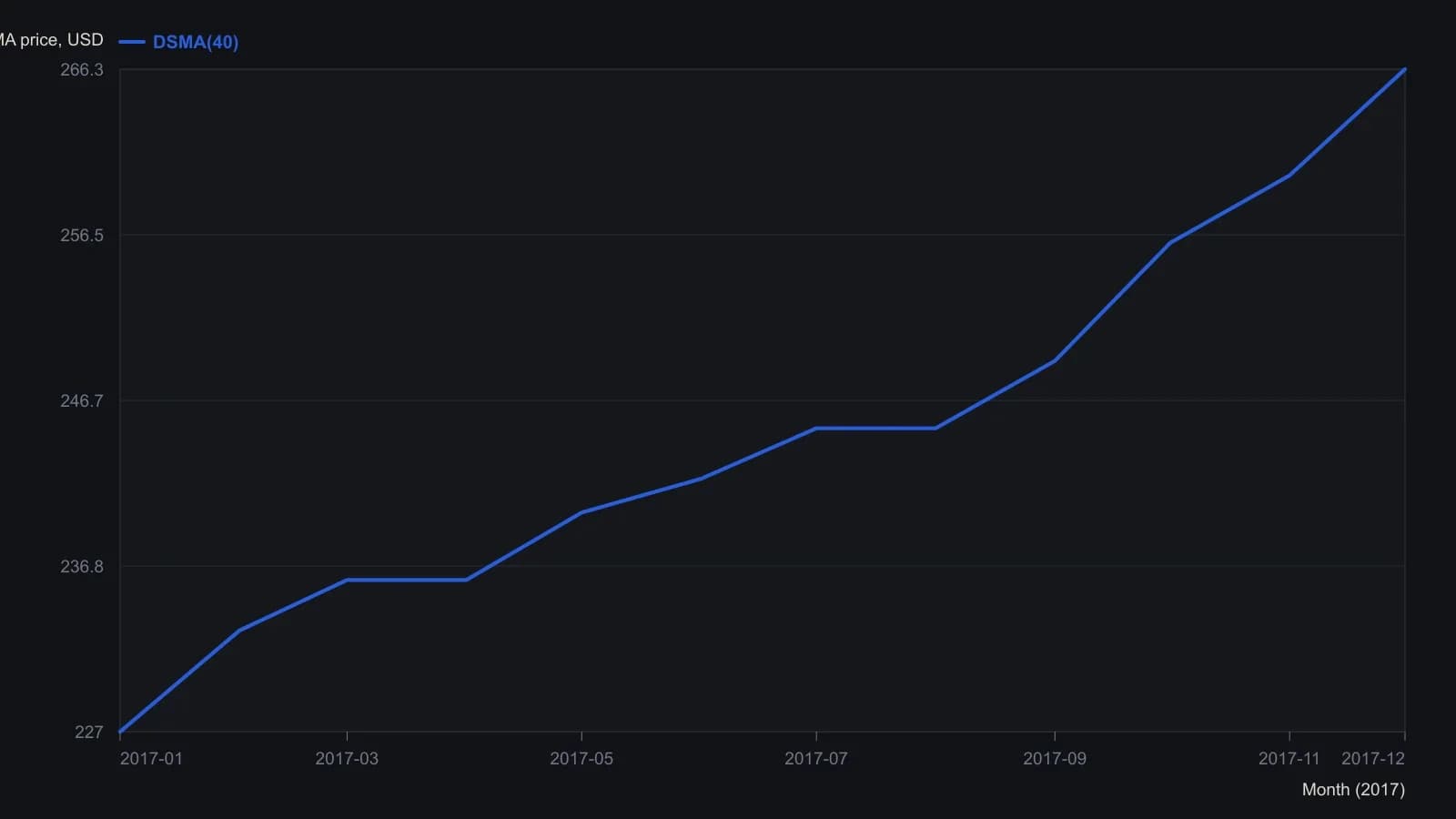
The raster is a magazine illustration of TradeStation Figure 1, not a data table. Points are month-end visual readings of the DSMA overlay; last printed DSMA(40) on the quote bar is 266.30. Do not treat tenths as exact ticks.
All readings on this track · 24 readings
- 1991Building variable-length moving averages from partitioned price changes
- 1991Variable-length moving average from change dispersion
- 1992Constructing volatility-adaptive exponential smoothing
- 1995Constructing an adaptive moving average with an efficiency ratio and filter
- 1995Two-gate breakout confirmation with adaptive averages
- 1995Building momentum-scaled adaptive moving averages
- 1995Adaptive length as a construction choice inside exponential smoothing
- 1998Testing price-channel breakouts with a lag-aware adaptive average
- 1998Constructing filters by nesting offsets and variable weights
- 1998Constructing an efficiency ratio adaptive average and entry filter
- 2001Encoding candle structure as a numeric filter
- 2001Adaptive averages driven by cycle-phase speed
- 2005Constructing an adaptive moving average from a fractal-dimension weight
- 2005Range-dimension adaptive exponential filter
- 2010Constructing simple, exponential, and adaptive averages
- 2010How a price-hugging smoother is assembled from ordinary averages
- 2013Evaluating an adaptive moving average against a same-window moving average
- 2016Three-layer confirmation: adaptive average, stochastic relative strength index, and stop-and-reverse
- 2017One-alpha reverse-path exponential smoothing
- 2018Pair two adaptive averages to filter swing turns
- 2018Two Adaptive moving averages as a confirmation pair
- 2018Constructing an adaptive filter for adoption-cycle reversals
- 2018Constructing a deviation-scaled adaptive moving average
- 2020Walk-forward and adaptive averages as two tests of the same trend