2005issue C101-7
Constructing an adaptive moving average from a fractal-dimension weight
This archive note shows how a recursive moving-average smoother takes its mixing weight from a fractal-dimension estimate of recent high-low range, then reuses that same adaptive function as the center of a band construct so an explicit adaptive baseline can be compared with a fixed-period counterpart.
- The adaptive average is a recursive mix of the current price and the previous filter value, with the mixing weight taken from a fractal-dimension estimate of recent high-low range.
- That estimate compares range-normalized high-low extent on two successive half-intervals with the same quantity on the full even-length window, using a base-two logarithm of those three quantities.
- The same adaptive function can serve as the center mean of a band construct and as the series whose squared deviations set the upper and lower envelopes.
- A comparative construction pairs the adaptive average with a fixed-period exponential average of the same length and treats a price cross of each line as the shared long-only test rule.
A recursive mix driven by range
The adaptive average is built as a recursive mix of the current price input and the previous filter value, with the mixing weight taken from a fractal-dimension estimate of recent high-low range. In this archive workflow the adaptive-moving-average is a recursive smoother whose weight is reset from that estimate rather than from a fixed lookback.
Until the bar count exceeds the lookback plus one, the filter is initialized to the current price rather than to the recursive update.
Half-intervals and the dimension estimate
The fractal-dimension is a scale comparison of high-low range on two half-intervals versus the full interval, used to set the smoother weight. The estimate compares range-normalized high-low extent on two successive half-intervals with the same quantity on the full even-length window, using a base-two logarithm of those three quantities.
A range-normalized-interval is the high-minus-low extent divided by the number of bars in that interval and is the raw input to the dimension estimate. The half-interval-split measures range on the first half, the second half, and the full window before combining those three quantities. The even-period-constraint requires that the full lookback be even so the series can be split into two equal half-intervals.
Turning the estimate into a smoothing weight
The smoothing-weight is the coefficient that mixes the current observation with the prior filter value after the dimension estimate is transformed and clipped. It is obtained by exponentiating a negative multiple of one less than the dimension estimate, then clipping the result so it stays inside a closed unit interval.
Weight-clipping bounds the transformed dimension so the recursive update cannot collapse to a zero or explosive coefficient.
Bands from the same adaptive function
A band-construct places upper and lower envelopes a chosen number of deviations around the adaptive mean. The same adaptive function can be reused as both the center mean and the series whose squared deviations define those envelopes.
The band strategy computes the envelopes from an end-of-bar midpoint-price, a lookback of 16, and two deviations above and below the adaptive mean, with a divisor that treats the window as either a full population or a sample. Midpoint-price is the typical price input formed from the high and low of the current bar.
Half-window entry and a named function
An alternative implementation avoids requiring the user to enter an even period by asking for the half-window length, doubling it for the full interval, and seeding the recursion with the midpoint-price once that full length is reached.
The same range-to-dimension-to-weight pipeline is factored into reusable box-count, dimension, and filter steps so the adaptive average can be called as a named function of period and a price series.
A fixed-period counterpart
A comparative construction pairs the adaptive average at lookback 40 with a fixed-period-exponential-baseline of the same length and treats a price cross of each line as the shared long-only test rule. That baseline is a constant-weight exponential average used only as a comparison object for the adaptive construction.
XOM daily FRAMA through the late-2004 range and early-2005 rally
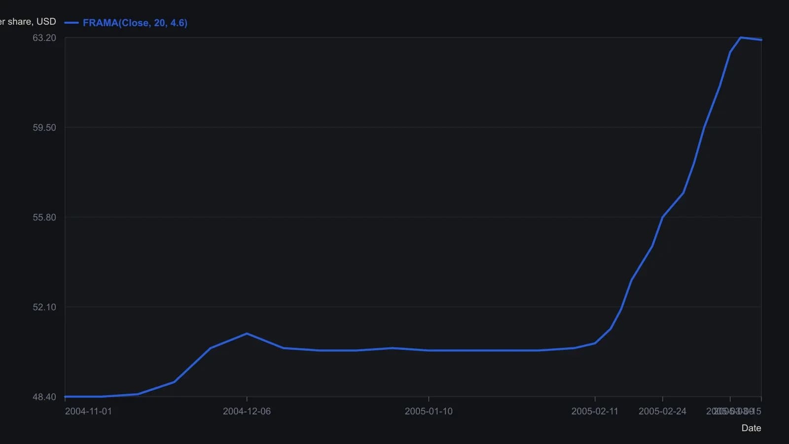
Source plots FRAMA of the close with a 20-bar window and Ehlers’ 4.6 exponential constant. Intermediate points are approximate tenths of a dollar from the raster; only the final 63.10 is printed on the figure. The five-day ROC pane was not carried over because it is a different unit.
All readings on this track · 24 readings
- 1991Building variable-length moving averages from partitioned price changes
- 1991Variable-length moving average from change dispersion
- 1992Constructing volatility-adaptive exponential smoothing
- 1995Constructing an adaptive moving average with an efficiency ratio and filter
- 1995Two-gate breakout confirmation with adaptive averages
- 1995Building momentum-scaled adaptive moving averages
- 1995Adaptive length as a construction choice inside exponential smoothing
- 1998Testing price-channel breakouts with a lag-aware adaptive average
- 1998Constructing filters by nesting offsets and variable weights
- 1998Constructing an efficiency ratio adaptive average and entry filter
- 2001Encoding candle structure as a numeric filter
- 2001Adaptive averages driven by cycle-phase speed
- 2005Constructing an adaptive moving average from a fractal-dimension weight
- 2005Range-dimension adaptive exponential filter
- 2010Constructing simple, exponential, and adaptive averages
- 2010How a price-hugging smoother is assembled from ordinary averages
- 2013Evaluating an adaptive moving average against a same-window moving average
- 2016Three-layer confirmation: adaptive average, stochastic relative strength index, and stop-and-reverse
- 2017One-alpha reverse-path exponential smoothing
- 2018Pair two adaptive averages to filter swing turns
- 2018Two Adaptive moving averages as a confirmation pair
- 2018Constructing an adaptive filter for adoption-cycle reversals
- 2018Constructing a deviation-scaled adaptive moving average
- 2020Walk-forward and adaptive averages as two tests of the same trend