1995issue C061-3
Constructing an adaptive moving average with an efficiency ratio and filter
The adaptive moving average is built to update slowly while price drifts sideways and quickly when price accelerates, reverses, or leaves a range. Construction uses an efficiency ratio, a squared smoothing constant, and a filter on successive adaptive-average changes to support first-signal-only buy and sell rules.
- Two n-period inputs, net change as direction and the sum of absolute one-period changes as volatility, form an efficiency ratio that equals 1 in a one-way window and approaches 0 when net travel is small relative to the path.
- A scaled smoothing constant interpolates a fast and a slow exponential speed with that ratio, then is squared so the adaptive weight nearly stalls when the window is mostly noise.
- Each new adaptive moving average value equals the prior value plus the squared constant times the gap to current price, after the first 10 observations are seeded with raw prices.
- A trend filter equal to a chosen percentage of the lookback standard deviation of successive adaptive-average changes, plus a first-signal-only rule, turns the long and short entries into one hold-until-opposite procedure.
What the line is built to do
The adaptive moving average is built to update slowly while price drifts sideways and to update quickly when price accelerates, reverses, or leaves a range. Construction starts from two n-period inputs and ends in a first-signal-only entry rule that holds until the opposite signal.
Editorial framing: TradersWeek reads this archive workflow as three layers. First, score how cleanly price traveled. Second, turn that score into a squared speed that almost freezes in chop. Third, wrap the line in a self-scaling band so the buy and sell rules can be audited as one procedure. That three-layer reading is editorial and is not attributed to the archive.
Score how cleanly price traveled
Construction starts from two n-period inputs. Price direction is the signed net change between the current observation and the observation n periods earlier. Volatility is the sum of absolute one-period price changes over the same n-period window, treated as a positive noise total. The worked window is 10 periods.
The efficiency ratio is direction divided by volatility. It equals 1 when every bar in the window travels the same way. It approaches 0 when net change is near zero relative to the path. In that sense the ratio is a cleanliness score: a one-way window sits at the top of the scale, and a back-and-forth window sits near the bottom.
Turn that score into a squared speed
Exponential speeds are converted with the mapping 2 divided by n plus 1. The example uses a 2-period fast constant of 0.6667 and a 30-period slow constant of 0.0645.
A scaled smoothing constant interpolates between those two speeds with the efficiency ratio, then is squared so the adaptive weight nearly stalls when the window is mostly noise. A high efficiency ratio therefore leans toward the fast constant. A low efficiency ratio leans toward the slow constant, and squaring pulls that already small weight still closer to a stall.
Each new adaptive moving average value equals the prior value plus the squared constant times the gap between current price and that prior value. The first 10 observations must be seeded with raw prices before the recursion is defined.
Wrap the line in a self-scaling band
The trend filter is a chosen percentage of the n-period standard deviation of successive adaptive-average changes. The worked percentage is 0.15. Small reversals that stay inside that band are ignored.
Rule-based entry uses only the first buy when the adaptive average exceeds its recent low by more than the filter, and only the first sell when the recent high exceeds the adaptive average by more than the filter. The position is held until the opposite signal. Later crossings in the same direction are not new entries.
Editorial note: because the band is a percentage of the variability of successive adaptive-average changes, it scales with the line itself. Combined with first-signal-only entry, the long and short rules become one procedure that can be audited from the same inputs. That audit reading is editorial and is not attributed to the archive.
Price and adaptive moving average from the sidebar worksheet
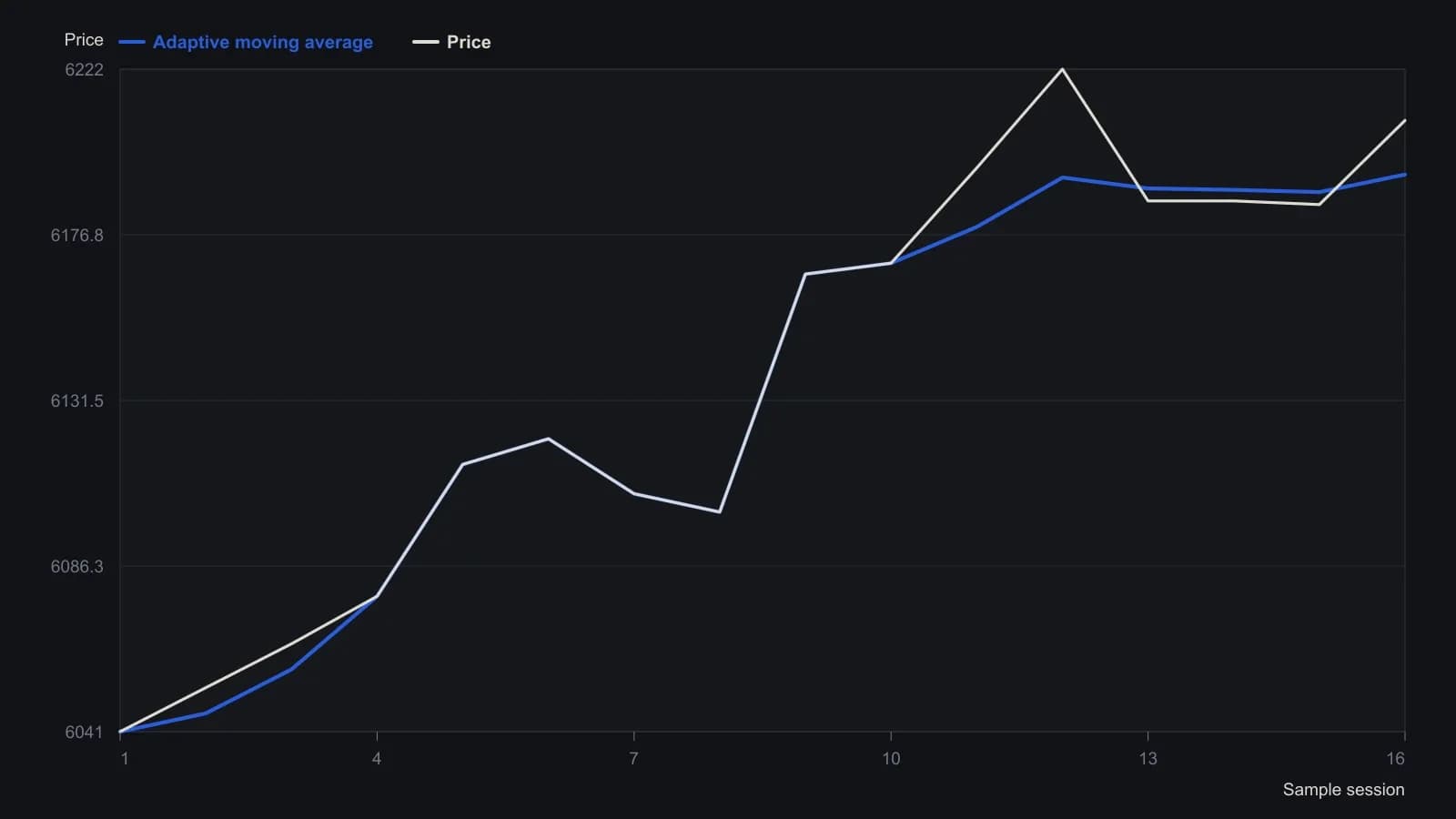
The first three date cells in the printed sheet all read 920603, so the x-axis is sample order rather than calendar time. Fast and slow smoothing constants are the 2-day and 30-day values 0.66667 and 0.0645; the filter uses 0.15 times the 10-day standard deviation of AMA changes. Rows 5–14 seed the average before the adaptive formula starts at row 15.
All readings on this track · 24 readings
- 1991Building variable-length moving averages from partitioned price changes
- 1991Variable-length moving average from change dispersion
- 1992Constructing volatility-adaptive exponential smoothing
- 1995Constructing an adaptive moving average with an efficiency ratio and filter
- 1995Two-gate breakout confirmation with adaptive averages
- 1995Building momentum-scaled adaptive moving averages
- 1995Adaptive length as a construction choice inside exponential smoothing
- 1998Testing price-channel breakouts with a lag-aware adaptive average
- 1998Constructing filters by nesting offsets and variable weights
- 1998Constructing an efficiency ratio adaptive average and entry filter
- 2001Encoding candle structure as a numeric filter
- 2001Adaptive averages driven by cycle-phase speed
- 2005Constructing an adaptive moving average from a fractal-dimension weight
- 2005Range-dimension adaptive exponential filter
- 2010Constructing simple, exponential, and adaptive averages
- 2010How a price-hugging smoother is assembled from ordinary averages
- 2013Evaluating an adaptive moving average against a same-window moving average
- 2016Three-layer confirmation: adaptive average, stochastic relative strength index, and stop-and-reverse
- 2017One-alpha reverse-path exponential smoothing
- 2018Pair two adaptive averages to filter swing turns
- 2018Two Adaptive moving averages as a confirmation pair
- 2018Constructing an adaptive filter for adoption-cycle reversals
- 2018Constructing a deviation-scaled adaptive moving average
- 2020Walk-forward and adaptive averages as two tests of the same trend