1984issue C021-9
Three-gate confirmation for wave, ratio, and cycle turns
A historical futures workflow splits a market reading into wave pattern, inter-wave Fibonacci ratios, and the time interval of the bull or bear swing. A turning-point hypothesis is treated as complete only when the wave count, a Fibonacci ratio objective, and a Fibonacci time cycle coincide. An unsatisfied category is scored as a discrete cut in certainty.
- Three-gate confirmation treats a historical futures reversal as a fully specified hypothesis only when wave-count completion, a Fibonacci ratio objective, and a Fibonacci time-cycle window coincide.
- A completed bull structure is three major up-waves separated by two major corrections, for five major legs. A bear structure keeps that same count even when the shapes differ.
- A missing-gate downgrade reduces certainty by the unsatisfied category when a Fibonacci time cycle is not clearly finishing, even if the wave count and a 1.618 ratio objective look complete.
- Fibonacci ratio objectives relate successive waves to their corrections with 0.618, 1.618, and the series' early 1:1 relation, while longer-horizon timing keeps 21-day through 144-day intervals in view as 3-week through 21-week cycles.
How the reading is decomposed
The method decomposes a market reading into three categories: wave pattern, inter-wave Fibonacci ratios, and the time interval of the bull or bear swing.
Editorial framing calls that joint rule three-gate confirmation. A turning-point hypothesis is complete only when wave-count completion, a Fibonacci ratio objective, and a Fibonacci time-cycle window all coincide.
Wave count before shape
A completed bull structure is specified as three major up-waves separated by two major corrections, for five major legs. A bear structure keeps the same count even if the shapes differ.
The wave count is a running tally of upward and downward swings used to judge whether a bull or bear structure has finished its required number of legs. The count is treated as more decisive than the visual shape.
Fibonacci ratio objectives
Each Fibonacci integer is the sum of the two preceding integers. Successive terms approach a 0.618 ratio or its 1.618 inverse.
Those ratios, plus the series' early 1:1 relation, are used to relate successive waves to their corrections. A Fibonacci ratio objective is a price target obtained by relating one swing to another with those successive-integer ratios.
Fibonacci time cycles
Longer-horizon timing uses 21-day, 34-day, 55-day, 89-day, and 144-day Fibonacci intervals, stated as 3-, 5-, 8-, 13-, and 21-week cycles. The 3-, 5-, 8-, and 13-day intervals are set aside for that longer-term focus.
A Fibonacci time cycle is a swing-to-swing interval taken from the Fibonacci integer series and used to mark when a bull or bear time window may expire.
When all three gates were specified together
The hog case set a third-wave downside objective at 40.50 as 1.618 times the prior down-leg. That price map coincided with an 89-week span from a December 1981 low and a 55-week span from the prior top.
The cattle case used a 233-week interval as the long-term timing frame and described the first major up-wave's correction as about 61.8 percent.
The silver case treated a 34-week interval from the low as a topping window and used 1.618 projections of 14.00 and 15.00 as confirming upside ratio objectives.
When the time cycle was not finishing
When no time cycle is clearly finishing, the Swiss-franc case treats certainty as reduced by that missing category even if the wave count and a 1.618 ratio objective appear complete. That cut is a missing-gate downgrade: certainty is reduced by exactly the unsatisfied category.
The wheat case placed a third-wave downside ratio objective at 3.15 from 1.618 of wave 1, while the next 55-week cycle was not due until early March, so the remaining gates were staggered.
Editorial reading: a wave extension is continuation of a supposedly finished third wave beyond the mapped ratio objective, which is why an incomplete time gate leaves the count open to further downside or upside travel.
The same ratio on different swings
The soybean case recorded three distinct 61.8 percent retracements during the downtrend. It distinguished a 61.8 percent measure of the July 1983 advance from a 61.8 percent measure of the entire rise from the October 1982 low.
Live hog futures, 1980–1984, with the October 1983 three-gate low
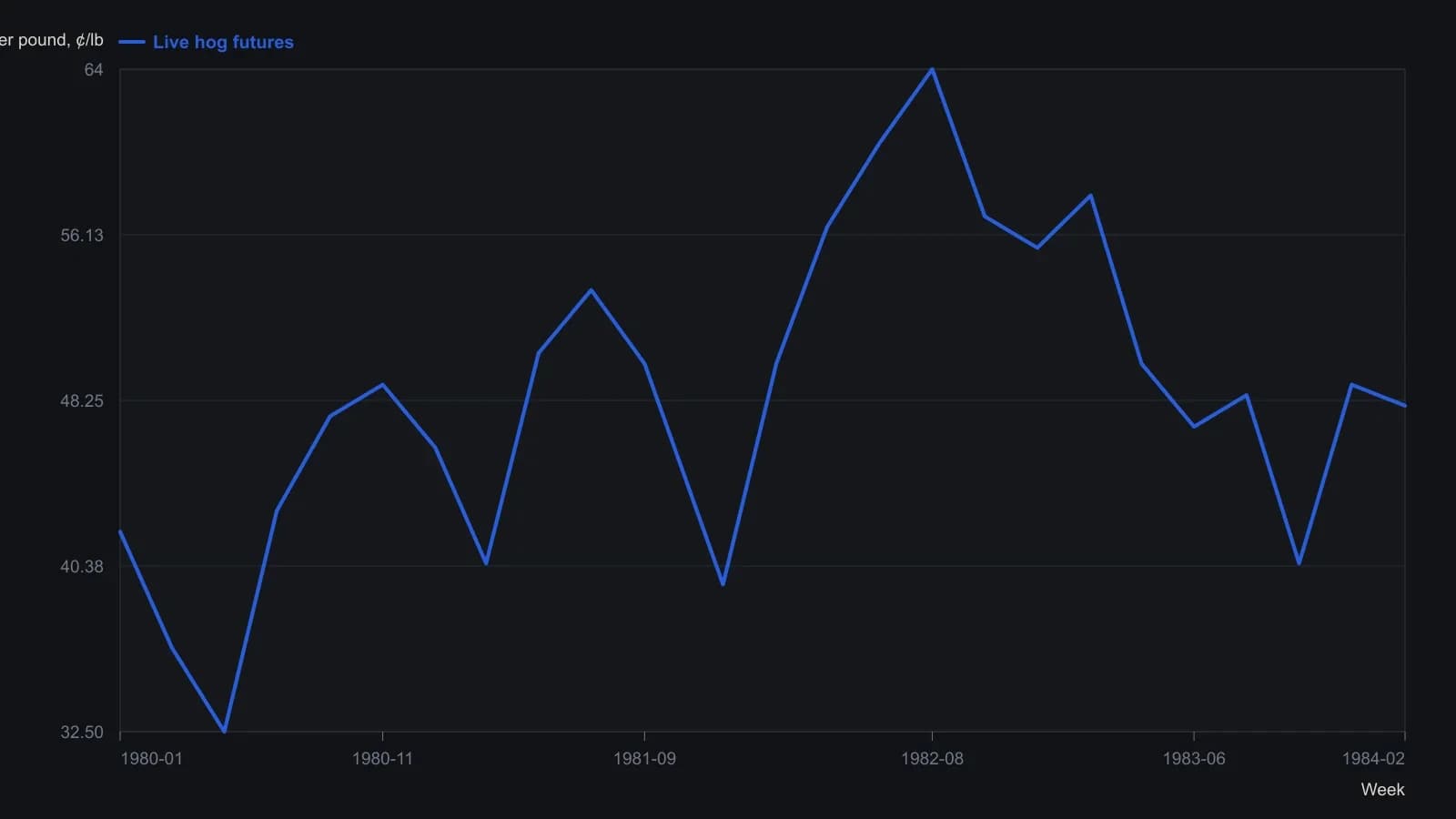
Prices are weekly closes digitized from the printed CRB grid, not a source table. The 40.50, 0.29, 0.46 and 0.68 levels, and the 89-week and 55-week spans, are the article’s stated figures and were used as anchors. No more than the readable weekly path is returned.
All readings on this track · 26 readings
- 1984Three-gate confirmation for wave, ratio, and cycle turns
- 1988Triaging Elliott wave counts with weekly stochastic divergences
- 1989Dominant-cycle phase flips as regime tests
- 1989Audit signals against elasticity regimes
- 1990When wave counts fail the exclusion test
- 1991Evaluating hourly DJIA growth-rate and velocity attractors
- 1996If a terminal fifth is rewritten, fail the first count
- 1998Mapping industrial-average swings with Fibonacci growth and retracements
- 1999Define the stop before the wave or the divergence
- 2001Form-first Elliott wave construction with phi
- 2006Wave count, channel floor, and Fibonacci bands after a correction
- 2007Impulse and correction as a recursive fractal recipe
- 2008Gold-silver ratio as a shoreline wave
- 2008A daily chart trend filter with Elliott wave abstention
- 2010Revising Elliott wave counts with RSI and stochastic guides
- 2010Constructing corrective-wave hypotheses with Fibonacci retracements
- 2011Pre-commit the wave-and-ratio stop before entry
- 2012Dated wave and ratio cases need a later-sample test
- 2013Keep a 1-2-3 count only while zigzag, Fibonacci depth, and divergence still agree
- 2014Elliott-wave target versus the option bid-ask
- 2014A three-layer classroom on one daily futures chart
- 2015Elliott wave classifies the swing; trend following holds the trade
- 2016Constructing wave labels and retracement zones from chart structure
- 2017Sector ETF pairs in quiet regimes
- 2017A policy-shift case that tested a delayed long-cycle wave count
- 2018One role each for wave, Fibonacci, and stochastic