1991issue C091-9
Evaluating hourly DJIA growth-rate and velocity attractors
A defined hourly DJIA lookback can test whether growth-rate counts and velocity basins behave like a quantitative baseline. Editorial contrast keeps Elliott wave analysis and Fibonacci retracement as conceptual overlays rather than as the measurement.
- Hourly DJIA observations from January 2, 1990 through February 15, 1991 were coded as up, down, or unchanged, with each day treated as seven continuous hourly points and changes of 2.5 points or less labeled unchanged.
- Labeled advances produced an aggregated up-to-down hour ratio of 1.672, and labeled declines produced an aggregated down-to-up hour ratio of 1.576, both noted as close to the Fibonacci ratio of 1.618.
- Growth-rate dynamics were summarized as two attractor basins near the golden mean, while hourly velocity showed several basins and a nonlinear, non-constant link to DJIA change.
- Editorial view: keep the hourly count and basin test as the quantitative baseline, and treat Elliott wave analysis and Fibonacci retracement as conceptual overlays rather than as the measurement.
The evaluation question
The study objectives were to inspect the fine statistical structure of hourly price changes and to test how far growth-rate and velocity variables could indicate the chance of daily and short-term DJIA changes.
Editorial reading: that aim is an evaluation question. A defined hourly lookback can be used to ask whether growth-rate counts and velocity basins behave like a quantitative baseline under Dominant cycle detection.
Hourly DJIA in the second half of 1989
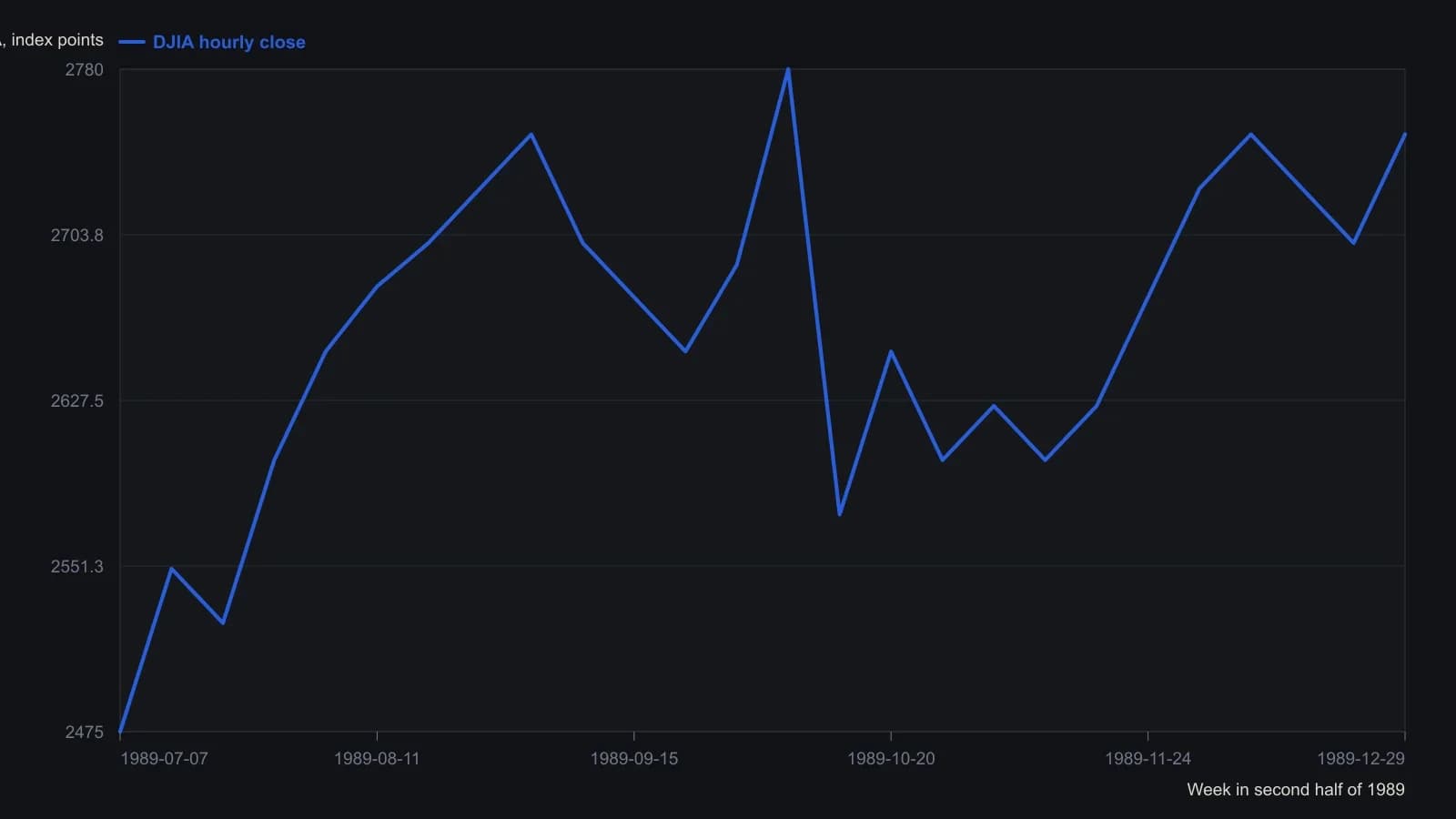
Raster digitization of weekly/hourly OHLC; y-values are approximate to the nearest 25–50 DJIA points and limited to the readable weekly spine.
How the hourly sample was coded
Hourly DJIA observations from January 2, 1990 through February 15, 1991 were coded as up, down, or unchanged. Each day was treated as seven continuous hourly points. Changes of 2.5 points or less were labeled unchanged.
Editorial note: that coding fixes the sampling interval and the lookback on which later hour counts and basin summaries depend.
Labels before a theoretical model
Short-term DJIA moves in that sample were first labeled by visual inspection of closes as up, down, or sideways, without using a theoretical model to define the segments.
Editorial contrast: those visual labels come before Elliott wave analysis or Fibonacci retracement. The overlays do not define the segments being counted.
Aggregated hour ratios
Across all labeled advances, 428 up hours and 256 down hours produced an aggregated up-to-down hour ratio of 1.672.
Across all labeled declines, 198 up hours and 312 down hours produced an aggregated down-to-up hour ratio of 1.576.
Those two aggregated hour ratios were noted as close to the Fibonacci ratio of 1.618. Sideways segments totaled 143 up hours and 127 down hours for a ratio of 1.126, nearer even occurrence of up and down hours.
Growth-rate and velocity basins
Growth-rate dynamics were summarized as two attractor basins near the golden mean. Time mediated the link between growth rate and DJIA change, so the length of a decline was related to how long down hours exceeded up hours.
Hourly velocity showed several attractor basins and a nonlinear, non-constant link to DJIA change. That link included stiffening that limited move size, softening that enlarged it, and a region of roughly linear velocity-to-magnitude behavior.
The October 13, 1989 DJIA break was presented as an exit from a linear uptrend into a non-proportional snap. Market action around October 10, 1989 was modeled as a broken-spring case of extreme softening.
What stays conceptual
Editorial practice: keep the hourly coding, the visual labels, and the growth-rate and velocity basins as the quantitative baseline. A later sample is the place for an out-of-sample check.
Elliott wave analysis and Fibonacci retracement can sit on the chart afterward as conceptual overlays. They should not replace the defined lookback or rewrite the segments after the counts are made.
All readings on this track · 26 readings
- 1984Three-gate confirmation for wave, ratio, and cycle turns
- 1988Triaging Elliott wave counts with weekly stochastic divergences
- 1989Dominant-cycle phase flips as regime tests
- 1989Audit signals against elasticity regimes
- 1990When wave counts fail the exclusion test
- 1991Evaluating hourly DJIA growth-rate and velocity attractors
- 1996If a terminal fifth is rewritten, fail the first count
- 1998Mapping industrial-average swings with Fibonacci growth and retracements
- 1999Define the stop before the wave or the divergence
- 2001Form-first Elliott wave construction with phi
- 2006Wave count, channel floor, and Fibonacci bands after a correction
- 2007Impulse and correction as a recursive fractal recipe
- 2008Gold-silver ratio as a shoreline wave
- 2008A daily chart trend filter with Elliott wave abstention
- 2010Revising Elliott wave counts with RSI and stochastic guides
- 2010Constructing corrective-wave hypotheses with Fibonacci retracements
- 2011Pre-commit the wave-and-ratio stop before entry
- 2012Dated wave and ratio cases need a later-sample test
- 2013Keep a 1-2-3 count only while zigzag, Fibonacci depth, and divergence still agree
- 2014Elliott-wave target versus the option bid-ask
- 2014A three-layer classroom on one daily futures chart
- 2015Elliott wave classifies the swing; trend following holds the trade
- 2016Constructing wave labels and retracement zones from chart structure
- 2017Sector ETF pairs in quiet regimes
- 2017A policy-shift case that tested a delayed long-cycle wave count
- 2018One role each for wave, Fibonacci, and stochastic