2000issue C111-6
Constructing adaptive channel breakouts from a measured cycle period
A channel-breakout construction can size entry and exit lookbacks as multiples of a Hilbert-estimated dominant cycle when fixed lookback inputs are left at zero. The same finished period then corrects the next bar's Hilbert amplitude error and is consumed by the matching signal's buy and exit orders.
- When fixed lookback inputs are left at zero, entry and exit lookbacks are sized as multiples of a Hilbert-estimated period.
- A two-dimensional Hilbert numbering scheme reduces computation but introduces quadrature amplitude error, which is offset with a straight-line term from the prior bar's frequency.
- A homodyne discriminator reads one-bar phase change as cycle length after the in-phase and quadrature pair is phase-advanced and smoothed.
- The finished period is change-limited, clamped between 6 and 50 bars, exponentially smoothed, and then reused by adaptive averages, sinewave indicators, and the matching channel-breakout signal.
A shared period estimate
The dominant cycle is the slowly varying market cycle length estimated from recent price observations and used to size subsequent calculations. In this construction the finished period is not a separate overlay. It is reused to compensate the next bar's Hilbert amplitude distortion, to drive adaptive averages or sinewave indicators, and to feed a simple channel-breakout signal.
A channel-breakout construction can size its entry and exit lookbacks as multiples of a Hilbert-estimated period when fixed lookback inputs are left at zero. Those windows are adaptive lookbacks: a channel or average length expressed as a multiple of the measured period instead of a fixed bar count.
S&P 500 with combined 34-day and 91-day cycles
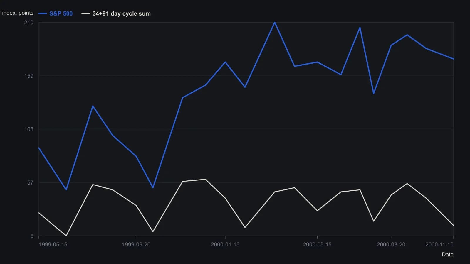
WAVEWI$E built Cycle1 as a 91-day @CYCLE anchored 28 January 1999 and Cycle2 as a 34-day @CYCLE anchored 10 August 1999; the lower green wave is their sum. The printed figure runs through mid-September 2000 and is extended forward to show the next scheduled trough. Values are digitised from the raster against the labelled 0–228.14 axis, so turning points are approximate and early-1999 candles are harder to separate from the cycle glyphs.
Smoothing and detrending before the transform
The period function first applies a four-bar weighted moving average, whose lag is described as one bar, then detrends the result. The detrend step is required because the Hilbert transform needs a detrended input.
In-phase and quadrature components
Fourier analysis, in this setting, is the decomposition of an ordered price series into in-phase and quadrature components so that the one-bar phase change can be read as cycle period. After a three-bar-lag quadrature calculation, the in-phase component is taken as the detrended series lagged three bars.
The pair is then phase-advanced and smoothed with an exponential average of alpha 0.15 before multiplication. Noise is reduced first, and only then is the complex product formed.
Reading period with a homodyne discriminator
A homodyne discriminator estimates period by multiplying the complex signal by its one-bar lag and reading the one-bar phase change as the cycle length. The multiplication produces a zero-frequency beat whose phase rate is that cycle length. The estimator is presented as preferable in a low signal-to-noise setting.
Compensating Hilbert amplitude error
A two-dimensional Hilbert numbering scheme that reduces computation also introduces amplitude error in the quadrature component. That error is offset with a straight-line compensation term taken from the prior bar's frequency. Amplitude compensation is this correction: it is applied so that a computationally cheap Hilbert transform does not distort the period estimate.
The prior-bar term is justified by the construction assumption that cycle period cannot change drastically from one bar to the next. The finished period is then written back into the next bar's compensation step.
Limits on the finished period
The finished period is change-limited, clamped between 6 and 50 bars, and exponentially smoothed. After those constraints it is reused to compensate the next bar's Hilbert amplitude distortion and to drive adaptive averages or sinewave indicators.
Sizing the channel from the same estimate
The matching signal is constructed as a simple channel breakout whose buy and exit orders consume the HilbertPeriod function output. When the fixed lookback inputs are left at zero, those orders inherit entry and exit lookbacks as multiples of the same Hilbert-estimated period.
The plotted Hilbert channel indicator is specified to use the same inputs and maximum reference-bar setting as the corresponding signal after those inputs have been optimized. The plot and the orders are therefore built from one period function rather than from a second, independent window.
All readings on this track · 26 readings
- 1982Critiquing Fourier, Elliott, and seasonal commodity models
- 1982Evaluating half-hour crossovers with cycle priors and stops
- 1984Building moving-window spectral cycle forecasts
- 1988Fourier cycles versus calendar seasonal regimes
- 1989Constructing analog cycle signatures from price lows
- 1990Curve fits fail the forecast test
- 1991Auditing moving-average length with Fourier spectra
- 1991Closed-form phase for dominant-cycle spectra
- 1993Evaluating windowed spectral forecasts of index turning points
- 1994Window length for moving-window spectral forecasts
- 1994Constructing WAMI power and phase spectra
- 1994Fourier-tuned momentum filter design
- 1994Aliasing, leakage, and dominant-cycle reads from sampled prices
- 1995Constructing indicator lookbacks from Fourier spectra
- 1996Constructing phase from a dominant-cycle sine and cosine pair
- 1999Sinusoidal pseudo-securities for indicator evaluation
- 2000Constructing dominant cycle length from Hilbert phase
- 2000Constructing adaptive channel breakouts from a measured cycle period
- 2005Embedding forex prices into a singular-spectrum forecast basis
- 2005Constructing recurrent forecasts from grouped spectral components
- 2007Constructing a dominant cycle from transformed Fourier spectra
- 2010Why cycle indicators fail when parameters shift
- 2019Constructing futures momentum as open-interest-scaled rate of change
- 2019Judging a dominant cycle and a trend filter by sample, lag and the move they keep
- 2020Constructing futures turnover time and urgency
- 2020Stock power ratio as a growth trend filter