1993issue C011-6
Evaluating windowed spectral forecasts of index turning points
The illustrated workflow forecasts index turning points from windowed Fourier components, scores every fitted period with frequency-domain ANOVA, and compares a reserved sample against a stated noise band.
- A univariate spectral procedure treats an index as one series, splits its history into frequency components, and recombines those components when cycles align instead of extending past price movement.
- The dominant cycle is the lowest-frequency repeating component that completes once per analysis window and should be ranked beside other periods rather than standing in for the whole spectrum.
- Frequency-domain ANOVA left 64.03% of variation across the rest of the spectrum after the two largest fitted components, so a method that keeps only a few periods is judged likely to fail as a forecast tool.
- The evaluation rule discards projected index changes of 2% or less on a reserved sample; the complementary cue is the next forecasted turn in the opposite direction, and path segments between turns are uninformative.
What the spectral procedure is doing
A univariate spectral procedure treats an index as one series whose unmodeled influences already sit in its history, then splits that history into frequency components that can be recombined when cycles align.
A turning point is defined as the approximate time a trend change occurs. Merely extending past price movement is treated as a misleading way to anticipate that change. Spectral analysis splits an ordered market series into frequency bands so each cyclical component can be measured, projected, and summed into a forecast.
In this workflow a turning-point is the approximate date when recombined projected cycles imply a change in the short-term trend.
Windows that let cycles change
Fourier analysis represents a price series as sinusoids tagged by period and frequency, plus a zero-frequency trend term that never repeats. Frequency-domain modeling treats the series as trend plus a spectrum of sinusoids. A 20-day component has frequency 1/20 cycles per day, and those components are allowed to evolve as a window advances.
Moving-window-spectral analysis slides a fixed-length subset along the series so each cycle's size and fit can be tracked as those cycles change. The illustrated analysis used 89 daily observations, an 82-day window, and eight successive windows stepping one day at a time from days 1 to 82 through days 8 to 89.
The dominant cycle is the lowest-frequency repeating component that completes once per analysis window, ranked beside other periods instead of standing in for the whole spectrum.
A scorecard for every fitted period
Frequency-domain ANOVA is a per-cycle split of explained versus residual variation, summarized with a coefficient of determination and an F ratio. Frequency-domain ANOVA attributes 2.15% of total variation to the non-repeating zero-frequency trend and 4.22% to the 82-day cycle that completes once per window.
The two largest fitted components account for 23.98% and 11.99% of variation (35.97% combined), leaving 64.03% across the rest of the spectrum, so a method that keeps only a few periods is judged likely to fail as a forecast tool.
Fit by cycle is judged with an F statistic whose 1% critical value is 13.74 (numerator df 1, denominator df 6). Frequencies 19 and 20 fall below that threshold, while most other listed periods, including grouped bands 21 to 30 and 31 to 41, do not.
Time-domain specifications that truncate or mask all but low-frequency cycles are presented as a reason those models often classify financial series as random walks, even though periodic alignment of many cycles can still produce a sharp turn.
DJIA cyclical variation by fitted period
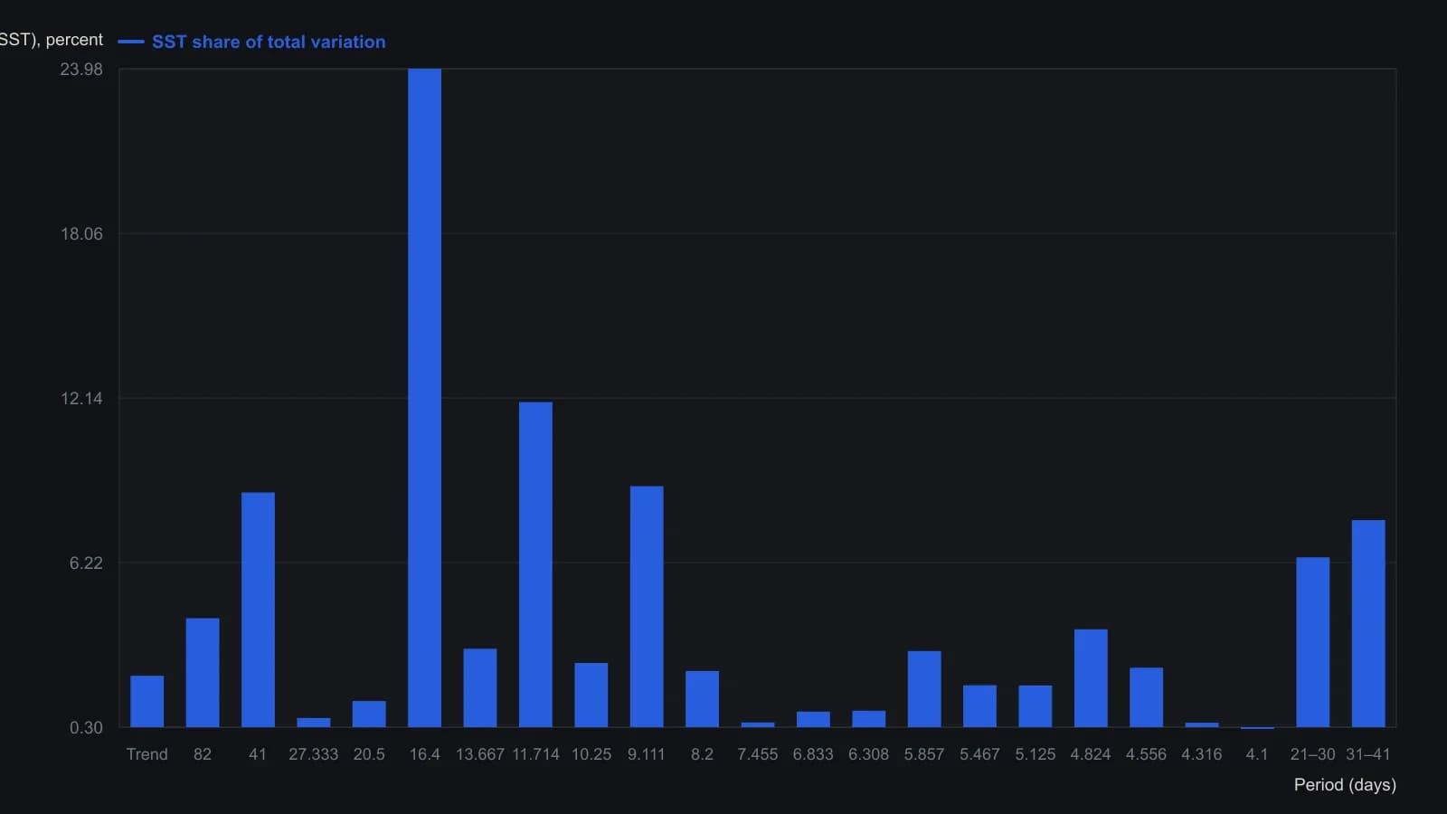
Ridley used 89 daily closes and an 82-day window stepped through eight positions (days 1–82 through 8–89). Frequencies 21–30 and 31–41 are grouped in the source. Critical F at the 1% level with (1, 6) degrees of freedom is 13.74; frequencies 19 and 20 fall below it.
Reserved sample, noise band, and the next opposite turn
The evaluation rule discards projected index changes of 2% or less. The worked example fitted only history through 12 December 1991 and reserved 13 to 26 December 1991 for comparison.
After a turning-point forecast, the complementary evaluation cue is the next forecasted turn in the opposite direction. Path segments between turns are treated as uninformative for judging the method.
All readings on this track · 26 readings
- 1982Critiquing Fourier, Elliott, and seasonal commodity models
- 1982Evaluating half-hour crossovers with cycle priors and stops
- 1984Building moving-window spectral cycle forecasts
- 1988Fourier cycles versus calendar seasonal regimes
- 1989Constructing analog cycle signatures from price lows
- 1990Curve fits fail the forecast test
- 1991Auditing moving-average length with Fourier spectra
- 1991Closed-form phase for dominant-cycle spectra
- 1993Evaluating windowed spectral forecasts of index turning points
- 1994Window length for moving-window spectral forecasts
- 1994Constructing WAMI power and phase spectra
- 1994Fourier-tuned momentum filter design
- 1994Aliasing, leakage, and dominant-cycle reads from sampled prices
- 1995Constructing indicator lookbacks from Fourier spectra
- 1996Constructing phase from a dominant-cycle sine and cosine pair
- 1999Sinusoidal pseudo-securities for indicator evaluation
- 2000Constructing dominant cycle length from Hilbert phase
- 2000Constructing adaptive channel breakouts from a measured cycle period
- 2005Embedding forex prices into a singular-spectrum forecast basis
- 2005Constructing recurrent forecasts from grouped spectral components
- 2007Constructing a dominant cycle from transformed Fourier spectra
- 2010Why cycle indicators fail when parameters shift
- 2019Constructing futures momentum as open-interest-scaled rate of change
- 2019Judging a dominant cycle and a trend filter by sample, lag and the move they keep
- 2020Constructing futures turnover time and urgency
- 2020Stock power ratio as a growth trend filter