2005issue C111-4
Constructing recurrent forecasts from grouped spectral components
Spectral forecasting can be audited as a construction. Choose a delay window, keep leading components, group similar oscillations, name the residual, then attach a linear recurrence and check where that recurrence cannot reverse.
- Choose the delay window first. Lengthen it for smoothing, shorten it toward the leading-component count when searching for hidden periods, and set it to a multiple of a known period when separating periodic fluctuations. The window should begin and end at roughly the same level.
- Rebuild from leading empirical orthogonal functions only. Average each elementary pattern of behavior along its skew diagonals to obtain reconstructed components, group similar oscillations, and treat the leftover gap as residual.
- Form the next value by linear recurrent continuation, using a predictor taken from the selected empirical orthogonal functions. That step cannot be applied when the squared elements of the last row of the right singular matrix sum to one or approach one, and it cannot reverse the local direction inherited from the window.
- If column means and scales were standardized so the trajectory matrix would fit a stationary decomposition, reverse those adjustments after reconstruction.
How the assembly is meant to be read
Spectral analysis, in this archive reading, is a decomposition of an ordered price, volume, or breadth series into leading components, grouped oscillations, and a residual so a reconstruction can be compared with the original path. Singular spectrum analysis is the delay-embedding method that rebuilds that series from empirical orthogonal functions of its trajectory matrix and can be limited to leading components for smoothing or continuation.
Editorial reading: treat the workflow as an assembly students can audit. Choose a delay window, keep only the leading components, group the cyclic leftovers, name the unused residual, attach a linear recurrence, and then inspect where that construction is structurally unable to reverse.
Choose a delay window
The delay window is the embedding length that sets how many lagged states enter the trajectory matrix and how many prior states the predictor later uses. Window length is a design choice. It is large when the aim is smoothing, shortened toward the leading-component count when searching for hidden periods, and a multiple of a known period when separating periodic fluctuations.
Fourier analysis enters at that last choice. It is a period-aware construction that ties the delay window to candidate cycle lengths so periodic, not necessarily harmonic, fluctuations can be separated after the leading components are isolated.
The selected window should also begin and end at roughly the same level.
Keep the leading components
A trajectory matrix built from ordered prices has constant values along its skew diagonals. That matrix can be fully rebuilt from its singular value decomposition. A usable reconstruction needs only the leading empirical orthogonal functions rather than the full set.
Singular value decomposition is the factorization that supplies those empirical orthogonal functions and their singular values. Leading components are the small set of empirical orthogonal functions tied to the largest singular values. They are the pieces used for a trend, a grouped oscillation, or a smoothing reconstruction.
Turn delay-space patterns into series
Each reconstructed matrix is an elementary pattern of behavior in delay space. It is reduced to a one-dimensional reconstructed component by averaging along the matrix skew diagonals.
The original series equals the sum of reconstructed components plus a residual. The first component is identified with a nonlinear trend at very high accuracy. Adding further components introduces oscillations. A larger collection of leading components nearly recovers the original path.
EURUSD hourly series rebuilt from leading SSA components
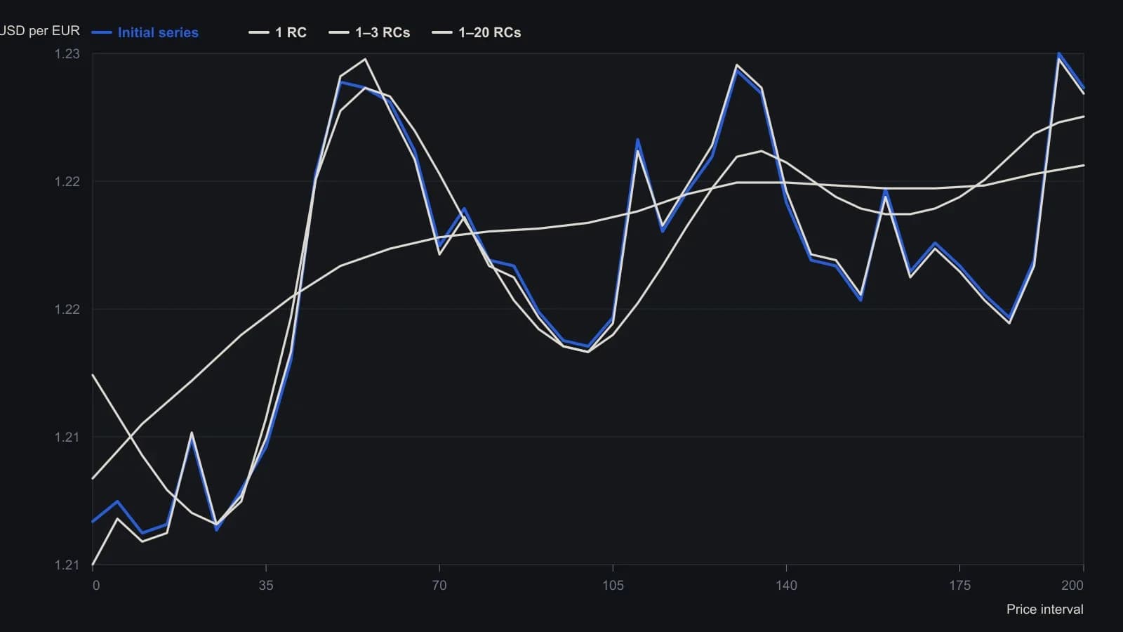
The source attributes about 99 percent of the leading singular value to the first component’s nonlinear trend. Delay window m and series length N are not printed on this pane. Turning points are only good to a few pips because the series were digitized from the plot, not copied from a table.
Group the cyclic leftovers
Reconstructed components can be grouped so that regular oscillations of similar amplitude or frequency are isolated. The archive illustration pairs neighboring components that share that cyclic structure and then recombines those groups with the trend component.
A principal component is only an intermediate projection. The matching reconstructed component does not store phase, amplitude, or frequency as direct attributes, so those traits are judged after reconstruction and grouping, not read off the projection itself.
Name the unused residual
The gap between the original series and a chosen reconstruction is treated as residual variation. The presented analysis assumes that residual is white noise.
Editorial reading: naming that unused remainder is how this article keeps the reconstruction auditable. Whatever was not placed in the trend or in a grouped oscillation stays outside the forecast construction.
Attach a linear recurrence
A next-step value is constructed by linear recurrent continuation. That value is a weighted combination of the previous delay-minus-one states. Those weights are stored in a predictor taken from the selected empirical orthogonal functions.
The predictor is the coefficient row, of length one less than the delay window, that supplies the continuation weights.
Inspect where continuation cannot reverse
Recurrent continuation cannot be applied when the squared elements of the last row of the right singular matrix sum to one, or approach one.
Linear continuation inherits the local direction of the chosen window. A segment with an upward tendency produces only upward continuation. It cannot generate a downward path from those same components.
Reverse any scale adjustment
Because the decomposition is formulated for stationary series, column means and scales of the trajectory matrix may be standardized before the singular-value step and must be reversed after reconstruction.
All readings on this track · 26 readings
- 1982Critiquing Fourier, Elliott, and seasonal commodity models
- 1982Evaluating half-hour crossovers with cycle priors and stops
- 1984Building moving-window spectral cycle forecasts
- 1988Fourier cycles versus calendar seasonal regimes
- 1989Constructing analog cycle signatures from price lows
- 1990Curve fits fail the forecast test
- 1991Auditing moving-average length with Fourier spectra
- 1991Closed-form phase for dominant-cycle spectra
- 1993Evaluating windowed spectral forecasts of index turning points
- 1994Window length for moving-window spectral forecasts
- 1994Constructing WAMI power and phase spectra
- 1994Fourier-tuned momentum filter design
- 1994Aliasing, leakage, and dominant-cycle reads from sampled prices
- 1995Constructing indicator lookbacks from Fourier spectra
- 1996Constructing phase from a dominant-cycle sine and cosine pair
- 1999Sinusoidal pseudo-securities for indicator evaluation
- 2000Constructing dominant cycle length from Hilbert phase
- 2000Constructing adaptive channel breakouts from a measured cycle period
- 2005Embedding forex prices into a singular-spectrum forecast basis
- 2005Constructing recurrent forecasts from grouped spectral components
- 2007Constructing a dominant cycle from transformed Fourier spectra
- 2010Why cycle indicators fail when parameters shift
- 2019Constructing futures momentum as open-interest-scaled rate of change
- 2019Judging a dominant cycle and a trend filter by sample, lag and the move they keep
- 2020Constructing futures turnover time and urgency
- 2020Stock power ratio as a growth trend filter