1984issue C051-10
Building moving-window spectral cycle forecasts
A moving-window-spectral construction estimates a frequency-response-function on a stationary windowed price series, inverts it into a convolution-forecast, and retains only projected turns that exceed an unsystematic-forecast-component allowance on reserved observations.
- Estimate numerical relationships among historical observations first, then apply those parameters to form future values of the same univariate price series.
- Remove or model trend and strictly periodic cycles so the windowed series meets stationarity, then advance a fixed-length window one observation at a time to manufacture spectral samples.
- Fit statistically independent frequencies one at a time, inverse-transform the frequency-response-function, and form a convolution-forecast with a systematic cyclical part and an unsystematic-forecast-component.
- Treat dominant-cycle alignment as an expected rise or decline only when the projected move exceeds the unsystematic-error allowance. The construction is aimed at direction changes, not pinpoint prices.
Estimate, then project
The spectral construction is a two-stage algorithm. Numerical relationships among historical observations are estimated first. Those parameters are then applied to form future values of the same univariate price series.
A moving-window-spectral procedure carries out that work in the frequency domain. It slides a fixed-length window along one ordered price series, estimates per-frequency parameters, and inverts them to form a forecast.
Least-squares time-domain parameter estimates are biased by autocorrelation. Lengthening the historical sample does not remove that bias.
Represent prices as cycles
In the Fourier-style frequency-domain-representation, prices are treated as sinusoidal cycles specified by frequency, magnitude, and phase. A component spanning 20 days is assigned a frequency of 1/20 cycles per day.
Manufacture windows that can be estimated
Because an economic series cannot be repeated as a controlled experiment, a window of predetermined length is advanced one observation at a time to manufacture additional windowed series for spectral estimation.
Trends and strictly periodic cycles are removed or modeled in the frequency domain so the windowed series can meet stationarity. Stationarity is the working condition of no systematic change in mean or variance. Once that condition holds, frequency components can be treated as independent.
Estimate a frequency-response-function
Once the windowed series is stationary, component frequencies are treated as statistically independent. Estimation proceeds frequency by frequency. The resulting frequency-response-function is inverse-transformed to the time domain.
Form the convolution-forecast
The forecast is formed by convolving past values of the series with the estimated parameters. That convolution-forecast is treated as a systematic cyclical part plus an unsystematic-forecast-component. The unsystematic-forecast-component is the residual portion attributed to measurement error, missing variables, and exogenous shocks rather than estimated cyclical structure.
In the worked construction, 100 daily industrial-average closes were split into 51 days for estimation and 49 days reserved for comparison. Estimation used one-day-differencing and 19 windows, with the level path recovered by inverse differencing.
Keep turns, not pinpoint prices
Grouped absolute forecast errors did not necessarily increase as the horizon lengthened, so the construction is aimed at identifying direction changes rather than pinpointing future prices.
When estimated component cycles are projected to align in one direction, the construction interprets that dominant-cycle alignment as an expected rise or decline, provided the projected move exceeds the unsystematic-error allowance.
Held-out MWS forecast errors cluster below 2 percent
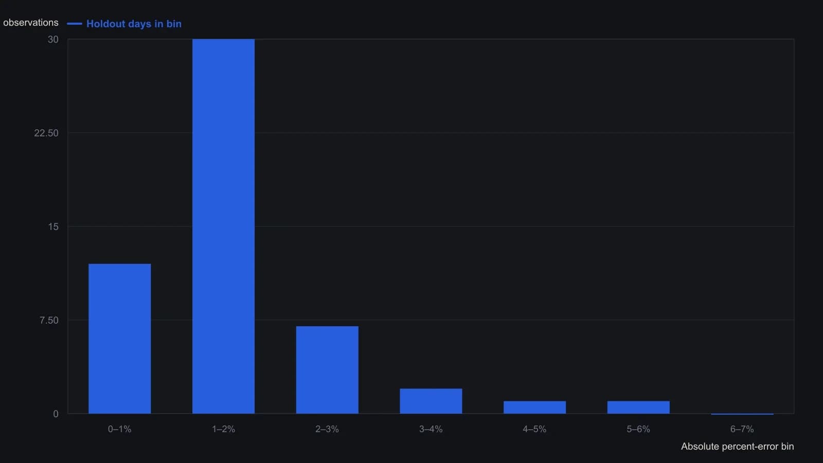
Ridley ignores the sign of each error and groups the 49 holdout days into 1-percent bins. He reports the 49-day percent MSE as about 2 percent and says those extra decimals should be rounded off. Heights are approximate readings from a coarse inverted scan and may be off by a count or two.
All readings on this track · 26 readings
- 1982Critiquing Fourier, Elliott, and seasonal commodity models
- 1982Evaluating half-hour crossovers with cycle priors and stops
- 1984Building moving-window spectral cycle forecasts
- 1988Fourier cycles versus calendar seasonal regimes
- 1989Constructing analog cycle signatures from price lows
- 1990Curve fits fail the forecast test
- 1991Auditing moving-average length with Fourier spectra
- 1991Closed-form phase for dominant-cycle spectra
- 1993Evaluating windowed spectral forecasts of index turning points
- 1994Window length for moving-window spectral forecasts
- 1994Constructing WAMI power and phase spectra
- 1994Fourier-tuned momentum filter design
- 1994Aliasing, leakage, and dominant-cycle reads from sampled prices
- 1995Constructing indicator lookbacks from Fourier spectra
- 1996Constructing phase from a dominant-cycle sine and cosine pair
- 1999Sinusoidal pseudo-securities for indicator evaluation
- 2000Constructing dominant cycle length from Hilbert phase
- 2000Constructing adaptive channel breakouts from a measured cycle period
- 2005Embedding forex prices into a singular-spectrum forecast basis
- 2005Constructing recurrent forecasts from grouped spectral components
- 2007Constructing a dominant cycle from transformed Fourier spectra
- 2010Why cycle indicators fail when parameters shift
- 2019Constructing futures momentum as open-interest-scaled rate of change
- 2019Judging a dominant cycle and a trend filter by sample, lag and the move they keep
- 2020Constructing futures turnover time and urgency
- 2020Stock power ratio as a growth trend filter