2006issue C061-4
Yield-curve spread as an equity regime filter
The Treasury curve is reduced to one long-minus-short spread and read in three states: ordinary positive, inverted, and unusually wide. That reading places a single equity holding in intermarket context instead of judging it only by its own price path.
- The yield curve is reduced to one yield-curve spread by subtracting the daily 13-week Treasury-bill yield from the daily 30-year yield.
- A positive spread is treated as the ordinary state because long-term holders take more interest-rate and inflation risk than bill holders. An inverted yield curve is framed as an abnormal near-term-risk regime.
- In a 1993-2006 sample, a moderate-positive band from 0.00 through +3.00 was the ordinary equity-holding regime. A negative spread or an overstretched positive spread was grouped as abnormal.
- Inversion aftereffects are described as a post-inversion window that typically lasts at least three months, including time after the spread has already turned positive again.
One spread from two Treasury yields
The yield curve is reduced to one yield-curve spread: the long-term Treasury yield minus the 13-week Treasury-bill yield. The spread is formed by first viewing the two yields as separate series, then subtracting the daily short-term yield from the daily 30-year yield.
A positive spread is treated as the ordinary state. Long-term holders take more interest-rate and inflation risk than short-term bill holders, so a long yield above the bill yield is the expected shape.
Inversion as an abnormal regime
An inverted yield curve is a negative spread in which short-term yields exceed long-term yields. That state is framed as an abnormal regime in which near-term risk is judged greater than distant risk, often around credit tightening or financial stress.
Inversion episodes listed for recent decades are 1966, 1969-70, 1973-74, 1979-81, and 2000-01. Each episode is described as accompanied or followed by equity bear-market conditions and short-run economic strain.
In the November 1993-February 2006 window, the only inversion began in July 2000 and ran through the first week of January 2001.
VTSMX weekly NAV through the 2000–01 inversion
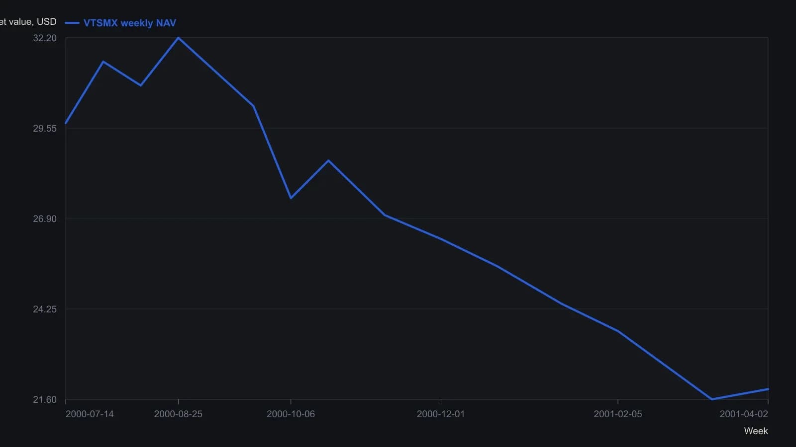
Closes were sampled from visible bar clusters rather than every weekly print; the raster does not support penny precision. The source states the inversion lasted July 2000 through the first week of January 2001, with the equity damage extending three months after the curve flipped back positive.
Ordinary and abnormal bands in one sample
For a 1993-2006 sample, equity exposure was classified as a moderate-positive regime when the spread sat between 0.00 and +3.00. That moderate-positive band is the ordinary equity-holding regime in the sample. Exposure was classified as an abnormal regime when the spread was negative or wider than +3.00. A positive spread wider than +3.00 is an overstretched positive spread and is grouped with inversion as an abnormal market state.
Those classified paths were then compared with an uninterrupted holding path. Aftereffects of inversion are described as typically lasting a minimum of three months, including time after the spread has already turned positive again. That weeks-to-months interval is the post-inversion window.
All readings on this track · 21 readings
- 1991A commodity-bond regime check before an equity relative strength index
- 1993A case study in refusing an isolated entry
- 1994The late-bull intermarket clock and regression-channel gates
- 1995Seasonal and political cycle maps as tested abstention regimes
- 2001Year-end high and low as a four-state regime filter
- 2002A six-market moving-average regime map from 2002
- 2003Gold as a regime marker after equity leadership fades
- 2003A four-season regime map before the shorter chart
- 2003From downtrend to trading range: implied volatility and volume after a shock fades
- 2006Exit discipline after regime shocks
- 2006Liquidity, growth, and midcycle market regimes
- 2006Yield-curve spread as an equity regime filter
- 2008Commodity, credit and bond alignment is not a forecast
- 2013Two lookback windows locate the cycle across bonds, stocks, and commodities
- 2014When ranging ends, replace the relative strength index, not its lookback
- 2016A Treasury-high-yield ratio as an equity regime filter
- 2016One-off shocks versus seasonal and secular regimes
- 2018Yield-curve flattening as missing market-regime context
- 2019Classifying six market phases around a single trade
- 2020Evaluating a two-window seasonal equity-bond switch
- 2020Dating energy regime breaks before the trade