1995issue C011-12
Seasonal and political cycle maps as tested abstention regimes
The archive described the year with a regime-overlay built from a seasonal-slice and a political-climate-map. A cycle-clock, a paired-tail-test, and a timing-multiplier then compared one abstention-rule with remaining fully invested.
- A regime-overlay maps the year before a standalone signal: seasonal-slice and political-climate-map coordinates classify which stretches are even eligible for a fully invested stance.
- A cycle-clock census put 32% of an average 39-month sequence in decline from a peak, 44% in reclaiming breakeven, and only 24% in new gains.
- A paired-tail-test and a timing-multiplier compared one abstention-rule with remaining fully invested through every month; turning-point precision was not required to match a fully invested rate.
- Seasonal-slice and political-climate-map readings sketched direction more than size, while indicator-rotation set which measure family led as the phase changed.
Map the year before issuing a signal
The archive used a regime-overlay to describe the expected shape of a year instead of issuing a standalone buy or sell. Intermediate-term work on the broad market could screen macro series with some statistical confidence, whereas single-name outcomes often hinged on events that resist quantification.
The cycle-clock spends little time in new gains
A cycle census back to 1885 put the average sequence at 39 months. Of that cycle-clock, 32% was spent declining from a peak, 44% reclaiming breakeven, and only 24% making new gains, so 76% of the clock was correction plus recovery.
A paired-tail-test of standing aside
In a monthly reconstruction since 1926, removing the 30 weakest months raised the long-run rate from 10.3% to 18.3%. Removing both the 30 strongest and the 30 weakest months moved it from 10.3% to 11%. That paired-tail-test, repeated for every equal count from 10 to 50 months, produced a 30% to 60% advantage versus remaining fully invested in the same reconstruction. The comparison frames one abstention-rule against staying invested through every month.
A timing-multiplier without precise turns
A capital-at-trough comparison found that sidestepping a 20% decline left 1.54 versus 1.00 on a fully invested path, and sidestepping a 10% decline left 1.26 versus 1.00. That timing-multiplier did not require turning-point precision. With 10% bull and bear cutoffs, missing 10.79% of each advance and each decline still matched a fully invested rate. With 20% swings the allowable miss was 20.63% at each end.
Seasonal-slice and political-climate-map
Daily percent changes since 1885 were read as a seasonal-slice by weekday and position in the month, rather than by reusing the same few days every month. Mondays were historically poor for being long and Fridays historically favorable. Place in the cycle, party control of the presidency and both legislative chambers, and the decade digit of the year were stacked into a political-climate-map. The yearly directional sketch was meant to describe the lay of the land, and was judged more useful for calling direction changes than for sizing moves.
Indicator-rotation through one cycle
The working process treated momentum, overbought or oversold conditions, monetary backdrop, seasonals, and short- versus long-horizon measures as rotating faces of one cycle. Indicator-rotation supplied the precedence scheme for which set leads in which phase.
Timing multiplier versus a fully invested dollar
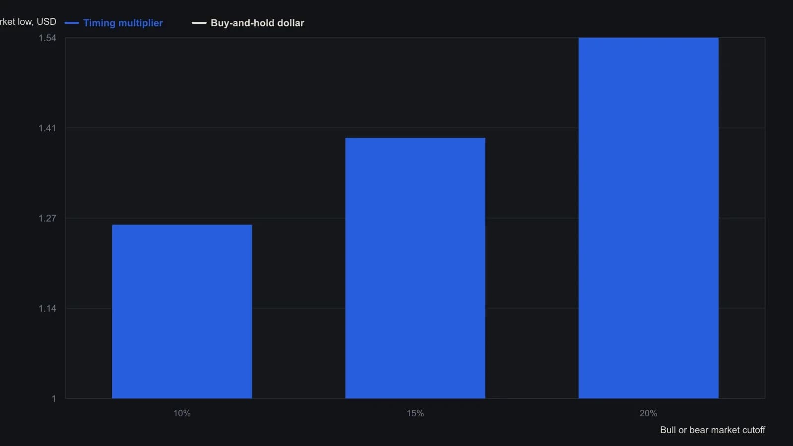
The source ignores dividends because both approaches earn them in bull markets, and it also omits interest earned on cash during bear markets. Multipliers are averages over market cycles since 1885.
All readings on this track · 21 readings
- 1991A commodity-bond regime check before an equity relative strength index
- 1993A case study in refusing an isolated entry
- 1994The late-bull intermarket clock and regression-channel gates
- 1995Seasonal and political cycle maps as tested abstention regimes
- 2001Year-end high and low as a four-state regime filter
- 2002A six-market moving-average regime map from 2002
- 2003Gold as a regime marker after equity leadership fades
- 2003A four-season regime map before the shorter chart
- 2003From downtrend to trading range: implied volatility and volume after a shock fades
- 2006Exit discipline after regime shocks
- 2006Liquidity, growth, and midcycle market regimes
- 2006Yield-curve spread as an equity regime filter
- 2008Commodity, credit and bond alignment is not a forecast
- 2013Two lookback windows locate the cycle across bonds, stocks, and commodities
- 2014When ranging ends, replace the relative strength index, not its lookback
- 2016A Treasury-high-yield ratio as an equity regime filter
- 2016One-off shocks versus seasonal and secular regimes
- 2018Yield-curve flattening as missing market-regime context
- 2019Classifying six market phases around a single trade
- 2020Evaluating a two-window seasonal equity-bond switch
- 2020Dating energy regime breaks before the trade