1998issue C051-4
Lagged phase clocks for market cycles
A historical workflow converted inflation-adjusted monthly industrial-average levels to logs, found dominant-cycle periods near 41 months and near 13 months, and plotted double-smoothed amplitude against delayed velocity. Editorial view: that two-axis state turns a Fourier period into a clock of late, early, and still-unconfirmed zones rather than a date to trade.
- Inflation-adjusted monthly industrial-average levels were converted to logs so equal percentage moves occupy equal distance before any cycle measurement.
- Dominant-cycle periods near 41 months and near 13 months set exponential-smoothing widths, and the amplitude-versus-velocity path stayed clockwise.
- The confirmed long-cycle diagram lagged by about 70 months, so a contrarian-strategy marked sells near 1:30 to 2:00 and buys near 7:30 to 8:00, before extremes could be known.
- The construction was described as poorly suited to noncyclical series, random walks, and single-name prices driven by firm- or industry-specific events.
Two delayed measurements
Inflation-adjusted monthly industrial-average levels were converted to logs so equal percentage moves occupy equal distance before any cycle measurement.
Editorial view: read the cycle as a delayed two-axis state. One axis is how far a double-smoothed series sits from a slow growth line. The other is how fast that gap is changing. A Fourier period then becomes a clock of late, early, and still-unconfirmed zones rather than a date to trade.
Dominant-cycle widths
Spectral inspection of that series located recurring periods near 41 months and near 13 months, which then set the double-smoothing widths for a long and a short motion. A dominant-cycle is a Fourier-identified recurring period used as the smoothing width for a long or short homeostatic motion.
Exponential-smoothing of level and speed
Exponential-smoothing, in this workflow, is repeated triangular moving averages that produce a double-smoothed level and a delayed velocity estimate so amplitude can be plotted against rate of change.
Long-cycle amplitude was the 41-month double-smoothed series minus a background real-growth line of about 1 percent a year. Velocity was monthly differences double-smoothed near 29 months and scaled to a yearly rate.
A clockwise phase-diagram
On the amplitude-versus-velocity plot the path always moved clockwise, with a larger swing drawing a larger loop and irregular price motion drawing an irregular loop. Homeostasis is that up-and-down motion, which keeps a circular phase structure even when the size, speed, and shape of each swing vary.
Logs of the real Dow, 1946–1996
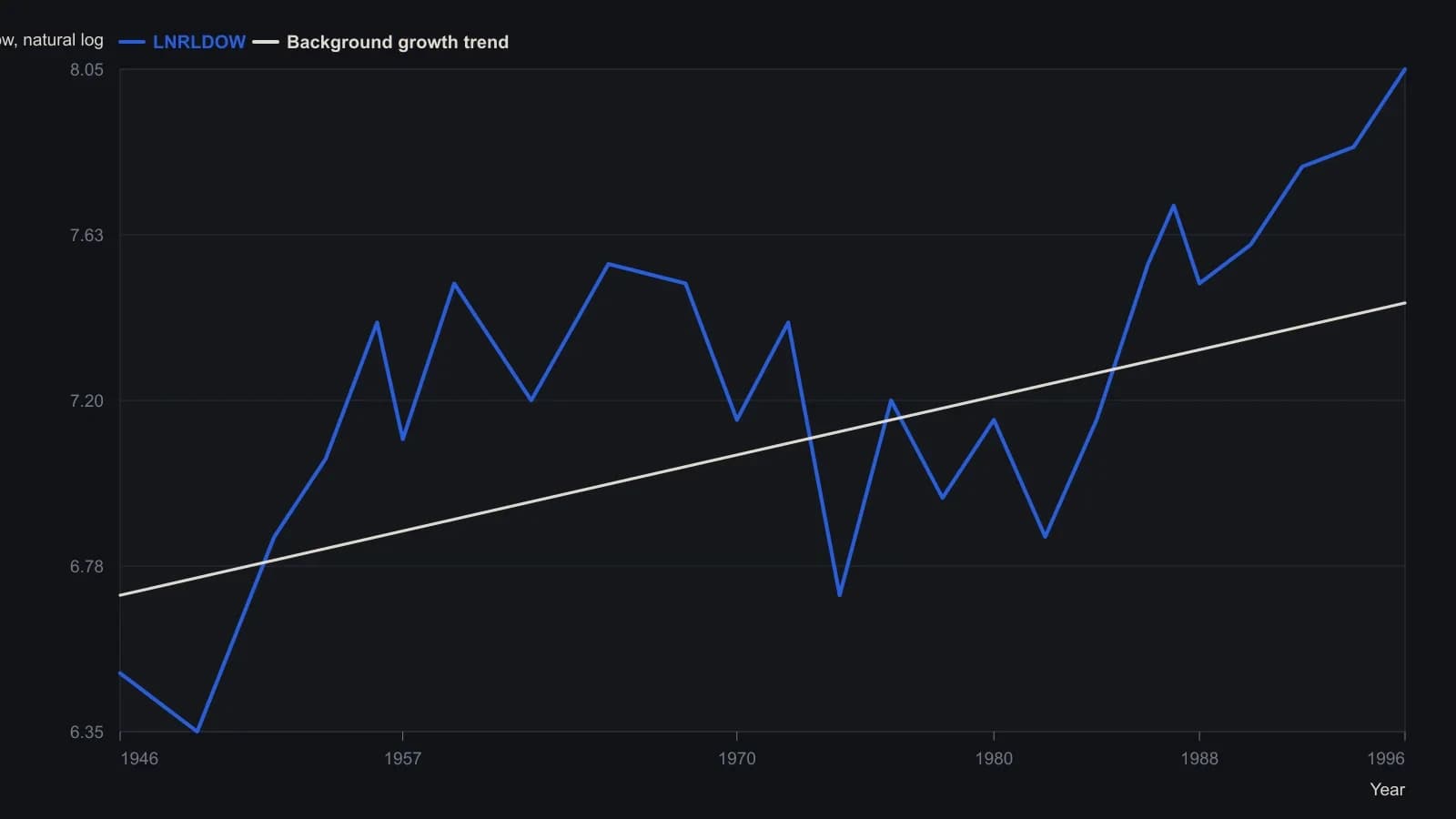
Figure 1 overplots LNRLDOW with the 41-month and 13-month triangular double-smoothed averages. Those two averages could not be separated from the monthly series at this raster resolution, so only the raw log series and the drawn growth line are returned. Years and log levels are approximate to about 0.05.
Phase-time on the lagged clock
An idealized phase clock placed the peak at 3:00, the trough at 9:00, the fastest rise at 12:00, and the fastest fall at 6:00, while noting those turning points are identified only after the averages become available. Editorial view: those hour marks locate late, early, and still-unconfirmed zones. They are not a calendar date for a trade.
Why the confirmed trace is late
Because the long-cycle velocity smoother needed about 29 months, the confirmed diagram lagged by about 70 months and the historical trace stopped near 1992. Phase-navigation is a trial estimate of the present point on a lagged diagram, used to read the risk of a swing before the moving averages are fully known.
A contrarian-strategy before the turn
The case-study navigation rule sold while the delayed clock still pointed before the peak, about 1:30 to 2:00, and bought while it still pointed before the trough, about 7:30 to 8:00, treating exact extremes as unknowable in real time. A contrarian-strategy here is that phase-clock rule: it marks sells while the delayed state still sits before a peak and buys only after the state has moved toward a trough, accepting that confirmation arrives after the turn.
Short-cycle state in mid-1987
Reconstructing the short-cycle state for mid-1987 placed it far to the right of the phase plot, which the study treated as a near-term downturn mark that the long-cycle state did not extend into a multi-year decline.
Series that do not fit
The same construction was described as poorly suited to noncyclical series, random walks, and single-name prices driven by firm- or industry-specific events.
All readings on this track · 20 readings
- 1986A pre-trade checklist for crowded trading methods
- 1988Contrary decision process versus lagging bullish consensus
- 1988Constructing contrarian signals from polled consensus
- 1989Constructing a ten-input breadth diffusion score
- 1989Even-number first penetration as a construction problem
- 1991Joint strength and sentiment rules for entries and exits
- 1995Evaluating contrarian sentiment thresholds for bond futures
- 1998A weekly composite-score that classifies despair, euphoria, or neither
- 1998Lagged phase clocks for market cycles
- 2003Process rules when a correct view fails
- 2003Closing stops and equity-curve filters as one decision process
- 2003One procedure for entry, exit, and standing aside
- 2004Cross-index volatility gauges as a premium regime map
- 2005When trend rules need a losing filter
- 2006Evaluating sector breadth as a contrarian regime filter
- 2011Sideline patience versus crowd noise
- 2012Assembling a sentiment zone oscillator as one contrarian filter
- 2012Currency regime context for fading rallies
- 2014When late trend confirmation is a sideline signal
- 2017Write a daily contrarian rule from the closed-end-fund discount