1992issue C101-9
Percent filters, log point-and-figure, and breadth residuals
A fixed point box does not scale with the price of an issue. This article writes the percent-reversal-filter and logarithmic-price-scale that make point-and-figure columns comparable, defines breadth as an advance-decline-residual, and only then applies a yates-corrected-chi-square to the binary hit-or-miss record.
- A one-point or three-point point-and-figure box filters out smaller increments, but that fixed point unit does not scale with the price of the issue.
- A percent-reversal-filter on a logarithmic-price-scale, with time on the horizontal axis, lets differently priced issues be compared without point-scale distortion.
- Breadth is written as an advance-decline-residual: the percent gap between an industrial average and the level implied by a regression on the adjusted-advance-decline-total.
- After fence-weeks are dropped, a yates-corrected-chi-square with one degree of freedom scores the remaining right-versus-wrong count against a coin-flip baseline.
Why a fixed point box fails
A one-point or three-point point-and-figure box filters out smaller increments, but that fixed point unit does not scale with the price of the issue.
On an arithmetic scale, a 5% move can be hidden near the bottom of a chart and look large near the top, and a straight arithmetic trendline implies a declining rate of advance.
A percent-reversal-filter on a logarithmic-price-scale
The construction replaces the point box with a specified percent-reversal-filter, plots price on a logarithmic-price-scale, and places time on the horizontal axis so differently priced issues can be compared without point-scale distortion.
A candidate turning point is drawn only as a provisional-reversal until a pullback of the specified percent confirms that the reversal has occurred.
One worked example records no move smaller than 10% and uses a logarithmic-price-scale so column height reflects percentage change.
Coca-Cola with a 10% reversal filter
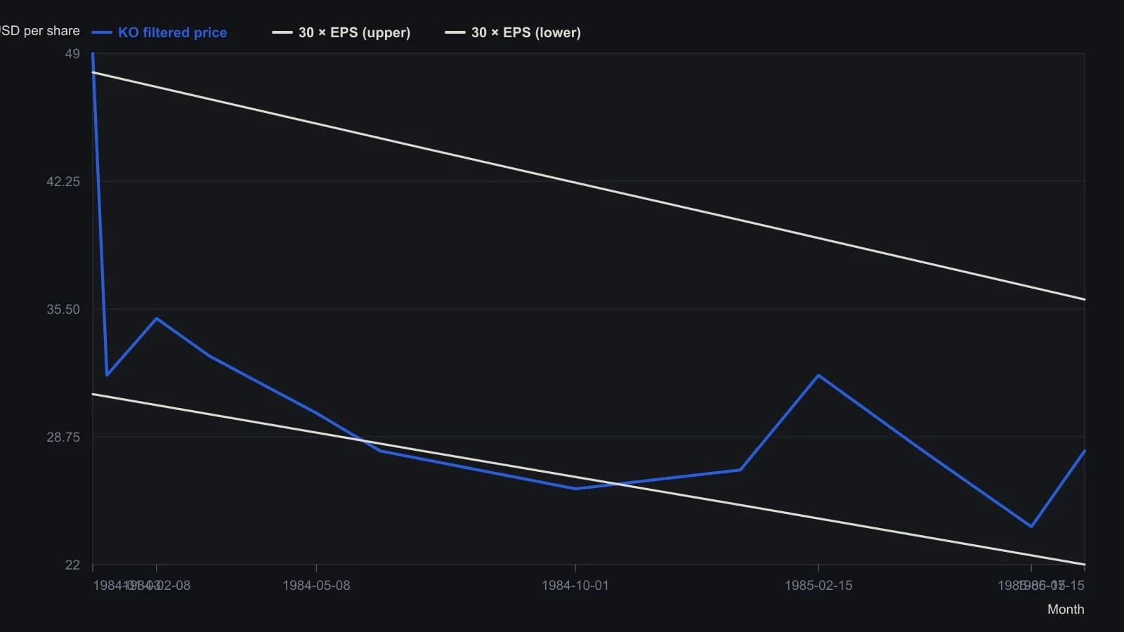
Reversals smaller than 10% are ignored. A turning point is drawn solid only after a pullback of that size. The printed vertical grid is equally spaced in dollars even though the sidebar argues for a logarithmic price scale.
Breadth as an advance-decline-residual
Daily breadth input is advances minus declines, divided by unchanged issues, accumulated, and then sampled at week-end for the oscillator. That running sum is the adjusted-advance-decline-total.
A one-year regression of an industrial average on that cumulative adjusted-advance-decline-total yields constants A and B. Expected level is A plus B times the current cumulative total, and the oscillator is 100 times the actual average divided by that expected level, minus 100.
Under that residual definition, a reading above 6% flags the average as high relative to breadth and a reading below 1% flags it as low relative to breadth. The percent gap is the advance-decline-residual.
A one-degree tally after fence-weeks
Each week is coded bullish, bearish, or on the fence. Later industrial-average direction is coded at 1, 5, 13, 26, and 52 weeks, and each fence-week is dropped from the right-versus-wrong count.
A yates-corrected-chi-square with one degree of freedom subtracts one from the absolute right-minus-wrong difference before squaring, then divides by the sum of rights and wrongs.
All readings on this track · 17 readings
- 1987Testing price-volume agreement after percent reversal filters
- 1988Constructing chi-square tests for two-way price counts
- 1988Building consensus indicators with correlation and the chi-square test
- 1988Test edges against chance, not story
- 1988Constructing an advance-decline divergence oscillator
- 1989Evaluate a contrary put-call premium ratio at a stated horizon
- 1990A weekly resistance-index from hourly volume-per-point
- 1990Testing breadth above moving averages by horizon
- 1990Evaluating member versus odd-lot breadth
- 1990A chi-square test of split frequency histograms across price aggregations
- 1990Evaluating smoothed secondary counts with a chi-square test
- 1991Treat session high and low times as codes, then require a chi-square check
- 1991A signed hourly swing catalog as a next-session chi-square check
- 1992Constructing a chi-square test as a gate for two-way market records
- 1992Percent filters, log point-and-figure, and breadth residuals
- 1997Build a chi-square stationarity screen before you forecast
- 1998Timed breakout rules after a nested-bar contraction