1992issue C091-10
Constructing clustered static and dynamic cycle forecasts
Static cycles keep a fixed interval between events, while dynamic cycles keep a constant proportion. The historical construction writes an explicit composite from pivot-point spans, projects those spans with both ratio families, and treats clustered dates and prices as the candidate windows for trend change.
- Markets are modeled as a composite cycle of several durations and amplitudes, so a cycle low need not coincide with the most obvious price pivot.
- Static cycles use a fixed interval between events, while dynamic cycles use a constant proportion, including the golden ratio of 1.618 and root ratios from a unit square.
- Every pairwise span among significant pivot points, taken over at least 100 observations, is multiplied by static and dynamic ratios and plotted forward to find projection clusters.
- The same ratio projections mark price swings, retracements, extensions, and support and resistance.
Write the composite baseline first
Markets are modeled as a composite of several cycles that differ in both duration and amplitude. The summed waveform is the composite cycle that later clocks are built to describe.
Adding three such cycles yields a summation in which a cycle low need not coincide with the most obvious price pivot. A pivot point is a significant change in trend used as the origin of an interval measurement.
Build a static clock and a dynamic clock
A static cycle is defined by a fixed interval between successive events. A dynamic cycle is defined by a constant proportion between successive events rather than a fixed gap.
A Fibonacci-style dynamic cycle is specified by a constant successive-term proportion of 1.618. That constant is the golden ratio, and the same 1.618 proportion can be drawn as a logarithmic spiral in which each section scales the previous section by that factor.
A unit square divided by successive diagonals produces a family of rectangles whose side ratios are the square roots of 2, 3, and 5. Those side ratios are the root ratios. The construction treats market dynamic cycles as the 1.618 proportion plus those root ratios, and treats static ratios as whole numbers together with quarter and third fractions.
Project every pairwise span
The procedure measures every pairwise span among significant pivot points over at least 100 observations. Each span is multiplied by the dynamic and static ratios, and the products are plotted forward on the time line.
Future dates where those projections cluster are treated as candidate windows for trend change. A projection cluster is such a window. When the hits come from more than one family of ratios, such as the 1.618 spiral, the root ratios, and the static fractions, the window is a multispiral cluster.
Mark price with the same ratios
The same ratio projections are also used to mark price swings, retracements, extensions, and support and resistance. Support and resistance here means price levels obtained by applying those static and dynamic ratios to swings so that retracements, extensions, and barriers can be marked.
Those price markings are illustrated on a June 1992 Treasury bond chart.
June 1992 Treasury bond futures, late 1990–January 1992
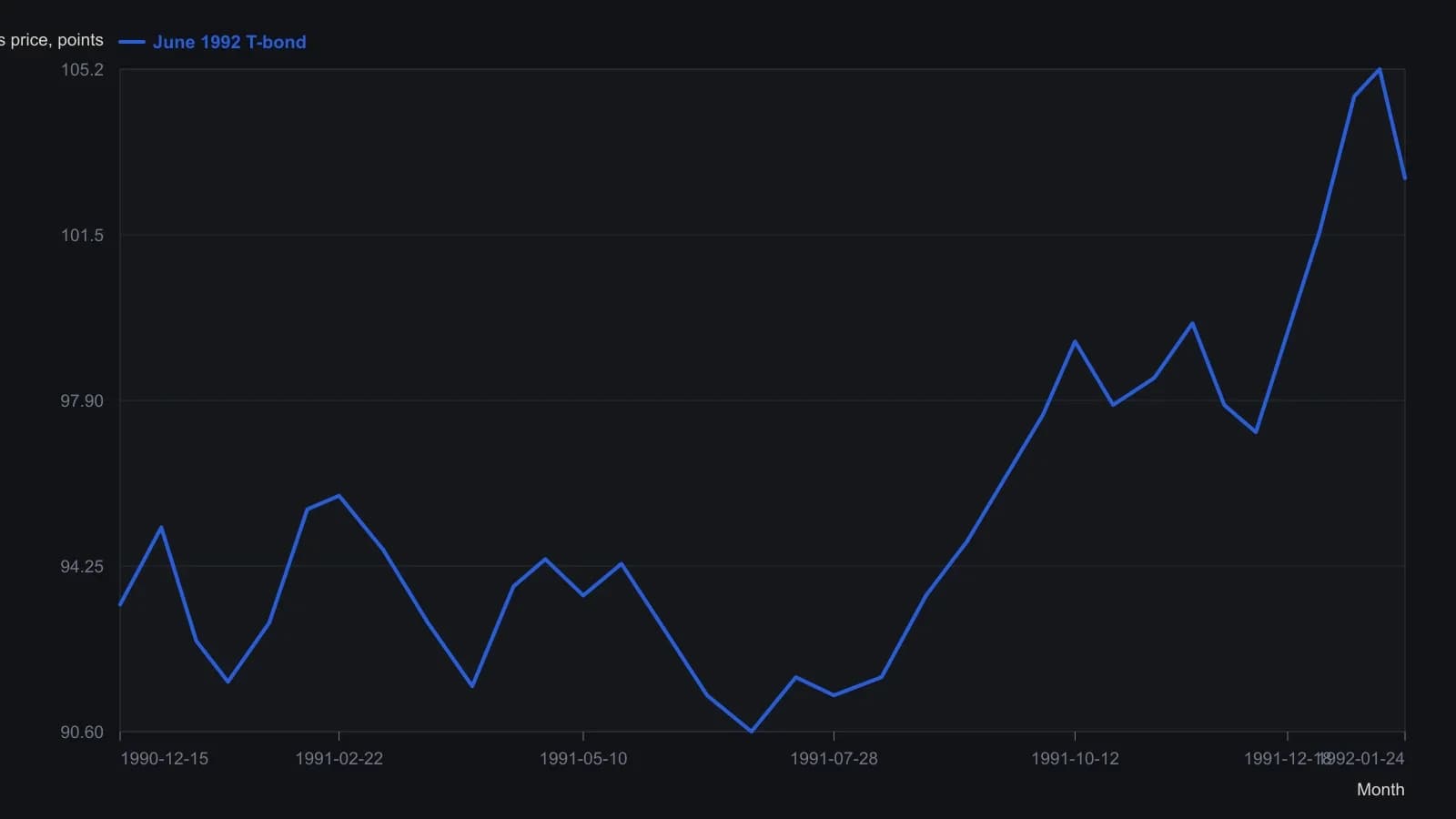
Prices are approximate readings from the printed grid (one-point spacing, 88–106). Root-3 and root-5 projections were omitted in the source. Digitized at roughly weekly resolution so the raster is not over-specified.
All readings on this track · 14 readings
- 1982A three-category Fibonacci filter for wave setups
- 1985Three-check Fibonacci swings in Treasury bonds
- 1990Elliott labels and Fibonacci day counts on a reversal-volatility plot
- 1991Constructing Fibonacci time-cycle clusters from wave ratios
- 1992Constructing clustered static and dynamic cycle forecasts
- 1992Constructing a five-cycle time-ratio workbook
- 1998Constructing support-resistance oscillators and Fibonacci time zones
- 2003Constructing nested fifth waves with Fibonacci ratios
- 2010Seasons, the Wall cycle, and Fibonacci time on a 1949 long wave
- 2011Building Fibonacci and Lucas time-cycle markers
- 2013Contracting Fibonacci time posts as a dominant-cycle classroom case
- 2013Classify the origin low before counting the next advance
- 2014Calling a cycle end with range bars, median lines, and Fibonacci
- 2015Building reaction zones with swings and median lines