1990issue C091-7
Elliott labels and Fibonacci day counts on a reversal-volatility plot
A constant-percentage reversal applied to every tick of the active stock-index futures contract can be joined into a reversal-volatility plot. Elliott labels and Fibonacci trading-day counts on that plot were used to date a window for volatility expansion, without a claim about the next cash-price direction.
- A fixed-percentage reversal of 0.77 percent, rounded to the nearest tick, turns successive flip points of the active stock-index futures contract into a reversal-volatility plot that keeps the same fraction at different price levels.
- The plot declines when swings sit between 0.77 percent and 1.54 percent and advances when wider swings dominate, whether those swings are up or down.
- Impulse, corrective, irregular, and triangle labels, and the trading-day spans between labeled lows, were read on the volatility series rather than on the cash price trend.
- Completion of the A-B-C correction was interpreted as a dated window for a strong rise in volatility in either direction, not as proof that a crash had to occur.
A reversal-volatility plot from a fixed-percentage rule
A volatility series can be drawn by applying a constant-percentage reversal to every tick of the active stock-index futures contract and joining successive flip points. The result is a reversal-volatility plot: consecutive flip prices joined so the net path of the reversal rule becomes the plotted line.
The illustrated reversal threshold is 0.77 percent of the latest high or low, rounded to the nearest tick. It is a fixed-percentage reversal, the same fraction of the latest extreme at different price levels, so the next hypothetical flip does not depend on the absolute index level.
Rollover from one active contract to the next is handled by a contract-rollover adjustment. The new contract's closing premium is added to the last extreme so the following 0.77 percent reversal can be computed on the successor contract.
When the plot rises and when it falls
The volatility plot declines when swings exceed 0.77 percent but stay below 1.54 percent. It advances when swings wider than 1.54 percent dominate, whether those swings are up or down.
Wave labels on the April-to-October plot
On the April-to-October 1987 plot, waves labeled A, B, and C spanned 14.9, 23.6, and 61.75 trading days, totaling 100.25 days. Those spans were described as near 100 times the Fibonacci ratios 0.146, 0.236, and 0.618.
Wave B was 1.42 times the vertical length of wave A and was labeled an irregular correction, a reading in which the B leg travels beyond the start of A and is taken as underlying strength in the volatility series. Wave C was labeled a triangle. Both readings were applied to volatility, not to the cash price trend. Impulse and corrective labels on the same plot, including the low of wave 2, were likewise applied to the reversal-built volatility series rather than to the cash price path.
Fibonacci trading-day spans
Trading-day spans between labeled lows and completed waves were compared with Fibonacci ratios and their multiples. The low of C and the low of wave 2 were 24.0 trading days apart. The a and e lows inside C were 33.2 days apart, presented as about 1.382 times that 24-day span.
Completion of the A-B-C correction was expected on the 100th trading day. That session showed repeated high-low swings just over 0.77 percent that pulled the plot down for the triangle's fifth leg.
A dated window, not a price direction
The wave-and-time structure was interpreted as a dated window for a strong rise in volatility in either direction, not as proof that a crash had to occur.
NYFE 0.77% reversal-volatility from April to October 1987
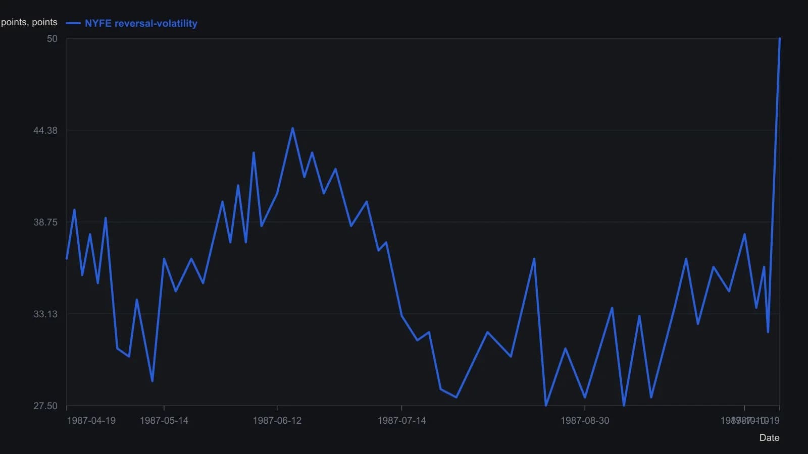
Williams fixed the reversal at 0.77% on every tick of the active NYFE contract and plotted trading sessions only (no weekend gaps); the September-to-December rollover on 9 September 1987 was shifted by a 1.85-point premium. Vertical ratios B = 1.42 × A and C = 1.58 × A are his stated guides. The curve was digitized to the nearest half-point.
All readings on this track · 14 readings
- 1982A three-category Fibonacci filter for wave setups
- 1985Three-check Fibonacci swings in Treasury bonds
- 1990Elliott labels and Fibonacci day counts on a reversal-volatility plot
- 1991Constructing Fibonacci time-cycle clusters from wave ratios
- 1992Constructing clustered static and dynamic cycle forecasts
- 1992Constructing a five-cycle time-ratio workbook
- 1998Constructing support-resistance oscillators and Fibonacci time zones
- 2003Constructing nested fifth waves with Fibonacci ratios
- 2010Seasons, the Wall cycle, and Fibonacci time on a 1949 long wave
- 2011Building Fibonacci and Lucas time-cycle markers
- 2013Contracting Fibonacci time posts as a dominant-cycle classroom case
- 2013Classify the origin low before counting the next advance
- 2014Calling a cycle end with range bars, median lines, and Fibonacci
- 2015Building reaction zones with swings and median lines