1991issue C031-7
Constructing Fibonacci time-cycle clusters from wave ratios
A change hypothesis is formed only when a time projection, a nearby price objective, and a pattern that implies change occur together. Time Cycle Ratio construction applies the same dynamic ratios used on price to completed time spans, then keeps a date only when several projections and mixed time counts fall inside a two-to-five-day cluster.
- Price-only study is treated as incomplete. A change hypothesis is formed only when a time projection, a nearby price objective, and a pattern that implies change occur together.
- Time Cycle Ratio construction measures a completed high-to-high or low-to-low span, multiplies it by ratios such as 0.382, 0.50, 0.618, 1 and 1.382, and counts those days forward from the span's end.
- A single Time Cycle Ratio date is not treated as sufficient. The method looks for a time-factor cluster inside a two-to-five trading-day window, typically two or three days.
- A dense cluster is not treated as proof of a reversal. Nearby Fibonacci retracement objectives and Elliott-wave pattern structure are used to judge the projected window.
Why price alone is treated as incomplete
Price-only study is treated as incomplete. A change hypothesis is formed only when a time projection, a nearby price objective, and a pattern that implies change occur together. That three-part test is the time-price-pattern coincidence rule.
Traditional fixed-length cycles are characterized as averages of past periods that mark only broad windows. The construction goal is to shrink the alert to a few trading days.
Elliott-wave ratios as the time template
Elliott-wave price-ratio projection between completed swings is presented as the template for time work. The same dynamic ratios used on price are applied to prior time cycles.
A Fibonacci time cycle is a completed high-to-high or low-to-low span multiplied by dynamic ratios such as 0.382, 0.50, 0.618, 1 and 1.382 and counted forward from the span's end to mark a candidate change window. Fibonacci retracement applies those same dynamic ratios to price swings to locate nearby support or resistance objectives that must sit inside the time window. Elliott-wave labeling is the swing-to-swing pattern check used to judge whether structure itself is signaling change inside a projected time cluster.
Building a Time Cycle Ratio
Time Cycle Ratio construction measures a completed span, multiplies it by 0.382, 0.50, 0.618, 1, 1.382 and related Fibonacci ratios, and counts that many days forward from the cycle's end. That proportioning step is the Time Cycle Ratio.
A 217-day Treasury-bond example
A Treasury-bond low-to-low span of 217 calendar days from 16 August 1988 to 21 March 1989, split at 0.382, 0.50 and 0.618, produced 83-, 109- and 134-day counts dated 11 June, 7 July and 2 August 1989, with nearby swing highs on 12 June, 11 July and 1 August.
Time Cycle Ratios of the 217-day T-bond low-to-low span
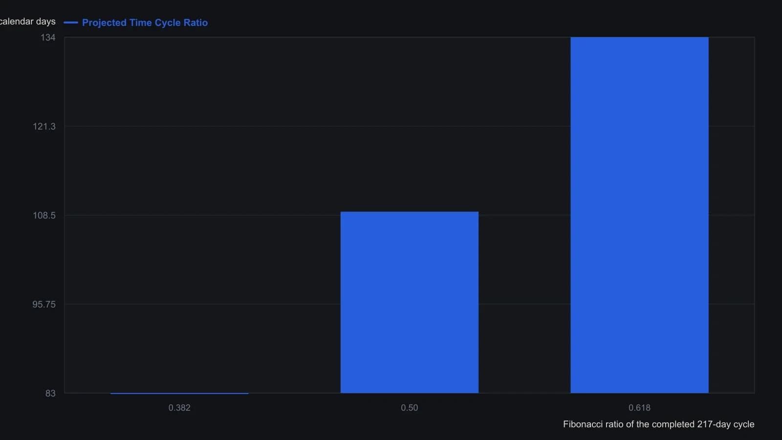
The article rounds 217 × 0.382, 0.50 and 0.618 to 83, 109 and 134 calendar days. The 11 June 1989 projection fell on a Sunday; the matching swing high was the next session, 12 June.
A cluster, not a single date
A single Time Cycle Ratio date is not treated as sufficient. The method looks for a cluster of several ratio projections and time counts inside a two-to-five trading-day window, typically two or three days.
Two or more independent time-ratio dates and calendar or trading-day counts that land inside the same one-to-five-session interval form a time-factor cluster. The short alert window that cluster creates is the projected turning-point period, often two or three trading days.
Composite time-count series
Time counts from important highs or lows use the Fibonacci series 3, 5, 8, 13, 21, 34, 55, 89 and 144, plus a composite set mixing those values with divisions of 144, 90 and 52, illustrated as 21, 30, 49, 60, 72, 90, 104, 144, 180 and 233 calendar or trading days. That mixed set is the composite time-count series.
A December 1989 cluster
Extending the 302-calendar-day span from the 19 October 1987 low to the 16 August 1988 low by 1.618 produced a 489-day count that landed on 17 December 1989 when projected from 16 August 1988. A peak followed on 20 December 1989.
The same December 1989 window also contained a 1.5 extension of the 1 August 1989 high to 26 September 1989 low, a 2.0 multiple of the 16 August 1988 low to 27 January 1989 high, plus 60 trading days from 26 September 1989, 144 calendar days from 1 August 1989 and 90 calendar days from 26 September 1989.
Judging the window after it arrives
A dense time-factor cluster is not treated as proof of a reversal. As price enters the projected window, nearby Fibonacci price objectives and Elliott-wave pattern structure are used to judge whether a top or bottom is forming.
All readings on this track · 14 readings
- 1982A three-category Fibonacci filter for wave setups
- 1985Three-check Fibonacci swings in Treasury bonds
- 1990Elliott labels and Fibonacci day counts on a reversal-volatility plot
- 1991Constructing Fibonacci time-cycle clusters from wave ratios
- 1992Constructing clustered static and dynamic cycle forecasts
- 1992Constructing a five-cycle time-ratio workbook
- 1998Constructing support-resistance oscillators and Fibonacci time zones
- 2003Constructing nested fifth waves with Fibonacci ratios
- 2010Seasons, the Wall cycle, and Fibonacci time on a 1949 long wave
- 2011Building Fibonacci and Lucas time-cycle markers
- 2013Contracting Fibonacci time posts as a dominant-cycle classroom case
- 2013Classify the origin low before counting the next advance
- 2014Calling a cycle end with range bars, median lines, and Fibonacci
- 2015Building reaction zones with swings and median lines